Topic Review (6 of 7): Fixed Income – Portfolio Management and Performance

The framework of fixed-income portfolio management and performance evaluation has undergone a quantitative revolution since the 1980s. Prior to this era, fixed-income management was primarily a simple, inactive buy-and-hold strategy focused on credit ratings and yield to maturity (YTM). Today, active trading, financial engineering, and complex instruments (such as securitized products and bonds with embedded options) require advanced analytical, statistical, and optimization methodologies to measure, monitor, and decompose portfolio risk and return.

1. Portfolio Yield Conventions and return metrics

To manage a portfolio effectively, analysts must first establish how to calculate portfolio yields and return metrics. The sources highlight several key approaches and their limitations:

Portfolio Yield:
- Weighted-Average Portfolio Yield: Calculated by weighting each individual bond’s YTM by its proportion of the portfolio’s market value. This is the most common but also most flawed method; it assumes a flat yield curve and parallel rate changes, failing to provide meaningful insight for asset-liability management (ALM) when bond maturities are highly divergent.
- Portfolio Internal Rate of Return (IRR): Calculated by aggregating all cash flows of the portfolio’s underlying securities and finding the discount rate that equates their present value to the total portfolio market value. While mathematically superior to the weighted average, it still suffers from traditional YTM drawbacks, such as the assumption that cash flows can be reinvested at the portfolio IRR.
Averaging Subperiod Returns: Realized portfolio returns are typically calculated for short subperiods (e.g., monthly) and then aggregated over the evaluation period using one of three techniques:
- Arithmetic Average Return: A simple, unweighted average of subperiod returns. This method is highly misleading; for instance, a portfolio that experiences a return in month one and a return in month two has a cumulative return of , yet the arithmetic average reports a misleading return.
- Time-Weighted (Geometric) Rate of Return: Measures the compounded growth rate of the initial portfolio value by taking the geometric average of subperiod returns. It is the preferred performance metric because it is unaffected by cash inflows and outflows (contributions and withdrawals) beyond the portfolio manager’s control.
- Dollar-Weighted Rate of Return: Represents the internal rate of return of all cash flows over the period. While useful for demonstrating overall fund growth, it is heavily distorted by the timing and size of client-driven cash flows, making it an unfair tool for comparing different asset managers.
Performance Presentation Standards: Ethical reporting guidelines (such as the CFA Institute standards) dictate that managers minimize the effect of external cash flows. Time-weighted returns calculated on a daily basis are preferred. If daily revaluation is not possible and an individual cash flow exceeds , the portfolio must be revalued on that date. Additionally, subperiod returns for evaluation horizons of less than one year should never be annualized.

2. Risk-Adjusted Performance Measures (Reward-Risk Ratios)

Comparing raw returns is insufficient; performance must be evaluated relative to the risk incurred to generate those returns. The sources analyze three primary ratios:

Sharpe Ratio: The ratio of a portfolio’s excess return (portfolio return minus the risk-free rate) to its standard deviation of returns.
- Limitations: It assumes returns are normally distributed. Because fixed-income returns are historically non-normal, asymmetric, and fat-tailed (due to downgrades and default events), the standard deviation penalizes upside volatility as a “risk,” which is inconsistent with investor preferences. Furthermore, it can be manipulated by changing the reporting window or shifting assets to risk-free cash at the end of a period to lock in a performance bonus.
Sortino Ratio: Addresses the Sharpe ratio’s limitations by measuring excess return relative to a client-specified Minimum Acceptable Return (MAR). It divides this excess return by the standard deviation of only those returns that fall below the MAR (measuring only “bad” or downside volatility).
Information Ratio: Measures a manager’s active return (alpha) relative to the backward-looking tracking error. The tracking error represents the standard deviation of the active return (portfolio return minus benchmark return). Generally, an information ratio between and is considered good, while a ratio of or higher over long horizons is exceptionally rare.

3. Portfolio Interest Rate Risk and Immunization

Managing interest rate risk requires aligning the sensitivity of the portfolio’s assets with its liabilities or benchmark index:

Portfolio Duration and Convexity: Portfolio duration and convexity are calculated as value-weighted averages of the durations and convexities of the individual bond holdings. Traditional portfolio modified duration assumes a restrictive parallel shift in the yield curve.
Shaping Risk: Because parallel shifts are rare, managers must measure exposure to nonparallel yield curve shifts (changes in slope and curvature). This is done using Key Rate Durations (measuring price sensitivity to a rate change at a specific maturity segment, holding other rates constant), Level-Slope-Curvature durations derived from Principal Component Analysis (PCA), or Yield-Curve-Reshaping Durations (SEDUR and LEDUR).
Bullet vs. Barbell Portfolios:
- A bullet portfolio concentrates maturities around the target investment horizon; a barbell portfolio splits holdings between short- and long-term maturities.
- The barbell portfolio possesses significantly higher positive convexity but a lower yield than a duration-matched bullet portfolio (the yield sacrifice is known as the “cost of convexity”).
- Under parallel shifts, the bullet portfolio outperforms the barbell for interest rate movements of less than 100 basis points due to its yield advantage. The barbell outperforms for larger rate movements due to the dominance of its convexity. However, under nonparallel shifts (such as a steepening of the yield curve), the bullet portfolio can dramatically outperform the barbell even across large rate shifts.
Macaulay Immunization: Classical immunization involves structuring a portfolio such that its Macaulay duration equals the target investment horizon, which perfectly offsets price risk and reinvestment risk under parallel rate shifts. Because duration changes with the passage of time and interest rate fluctuations, the portfolio must be periodically rebalanced, weighing the costs of rebalancing transactions against the risk of duration drift.
Contingent Immunization: A hybrid active-passive strategy. As long as the portfolio’s value remains above a specified “safety net” (representing the present value of the target terminal value discounted at the current immunizing rate), the manager can actively manage the portfolio. The difference between the active return and the required return is the cushion spread. If the safety margin is entirely eroded and hits zero, the manager must immediately immunize the portfolio to secure the target return.

4. Performance Attribution Analysis

To identify exactly how a manager achieved their active return, portfolio performance must be decomposed using Performance Attribution Analysis. The three primary approaches are:

Holdings-Based Attribution: Relies on beginning-of-period holdings and reflects a buy-and-hold strategy over the evaluation period.
- Sector-Based Models: Traditionally utilize variants of the equity Brinson model, adjusting for duration weights. However, applying equity models to fixed-income can be highly misleading, as they fail to distinguish between true sector allocation and duration exposure.
- Factor-Based Models: Decompose excess returns into risk factors such as yield curve changes (shift, twist, butterfly), spread changes, and income carry.
- The Campisi Model: A widely used model that decomposes total return into income-return and price-return effects. The price return is then attributed to the Treasury/duration effect (which can be further split into parallel shift and nonparallel twist effects using key rate durations), the spread effect, and a residual selection effect.
- Advanced Models: The Fong-Pearson-Vasicek model separates the external interest rate environment from active management skills (duration/maturity, spread/quality, and specific issue selection). The Kahn multifactor model isolates roll-down/carry and curve changes (shifts, twists, and butterfly adjustments). The Dynkin-Hyman-Konstantinovsky model applies option-adjusted spread (OAS) techniques to accurately handle curve-sensitive derivative exposures.
Transaction-Based Attribution: Captures intraperiod trading activity. While theoretically more accurate than holdings-based models, its extensive data requirements are costly and often do not provide a significant marginal improvement in accuracy over short subperiods.
Returns-Based Style Analysis (RBSA): Developed by William Sharpe, this is a low-cost, holdings-free statistical approach. It uses multiple linear regression of historical portfolio returns against a set of liquid, passive strategy indexes (such as bond trend, bond carry, FX volatility, FX carry, and rate volatility) to estimate the portfolio’s style exposures and active value added.

5. Systematic Portfolio Construction and Optimization

In modern fixed-income management, portfolios are built systematically using Multifactor Risk Models in conjunction with mathematical optimizers.

The Objective: The optimizer identifies the exact weight of each security to hold in order to minimize the portfolio’s forward-looking (predictive) tracking error relative to a designated benchmark.
Constraints: Optimization is performed subject to stringent client guidelines, risk budgets, transaction costs, turnover limits, and regulatory constraints (e.g., maximum exposure per issuer, sector limits, and specific duration or spread duration matching).
Robust Optimization: To combat estimation error in expected returns and risk parameters, managers utilize robust optimization, which models uncertainty using pre-specified confidence intervals. This technique helps prevent extreme portfolio concentrations, limits turnover, and stabilizes portfolio weights in the presence of transaction costs.

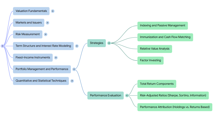
Strategies

The formulation and execution of fixed-income portfolio strategies have evolved from a historical reliance on simple buy-and-hold methodologies into a rigorous, quantitatively driven discipline. Today, portfolio managers navigate a broad spectrum of strategies designed to either match the performance of a market benchmark or secure a stream of cash flows to fund specific liabilities.

These strategies exist along a continuum, categorizing themselves into distinct passive, enhanced, and active frameworks.

1. The Passive and Enhanced Indexing Spectrum

When a portfolio is managed relative to a bond market index, the manager’s chosen strategy dictates the level of accepted tracking risk. The primary strategies along this passive-to-active spectrum include:

Pure Bond Indexing (Full Replication): The objective is to construct a portfolio that perfectly replicates the benchmark index by holding all of its constituent bonds in their exact index proportions. However, because the global bond universe is massive and contains thousands of highly illiquid, infrequently traded corporate and structured issues, full replication is rarely pursued due to its prohibitively high transaction and maintenance costs.
Enhanced Indexing by Matching Primary Risk Factors: To avoid the high costs of pure replication, managers utilize a sampling approach. This strategy constructs a representative portfolio of bonds designed to match the benchmark’s primary risk factors—such as portfolio duration, key rate durations, sector weights, and quality spread contributions. By aligning these key exposures, the portfolio’s return matches major market movements while significantly reducing transaction expenses.
Enhanced Indexing by Minor Risk Mismatches: This strategy maintains duration neutrality relative to the index but permits small, deliberate tilts in other factors—such as sector weights or quality categories—to generate a modest return premium. The goal is to generate enough outperformance (active return) to offset the portfolio’s administrative and management fees.
Volpert’s Five Index Enhancement Strategies: Because a passively indexed portfolio naturally underperforms its paper benchmark by the amount of its operating and transaction costs, enhanced indexers utilize five tactical methods to recover these costs:
1. Lower Cost: Maximizing net returns through tight controls on trading commissions, execution costs, and re-bidding advisory fees.
2. Issue Selection: Selecting individual bonds that are independently identified as undervalued relative to a valuation model’s theoretical price, often bypassing ratings agencies to perform in-house credit analysis.
3. Yield Curve Positioning: Exploiting structural pricing anomalies along the curve (such as consistently overvalued or undervalued maturity sectors) to capture yield advantages.
4. Sector and Quality Positioning: Maintaining a yield tilt toward short-duration corporate bonds (which historically offer the highest yield spread per unit of duration) or periodically rotating sector exposures.
5. Call Exposure Positioning: Underweighting premium callable bonds when interest rates decline to insulate the portfolio from the yield compression and cash-flow truncation associated with call risk.

2. Active Portfolio Strategies

Active fixed-income portfolio management is built on the premise that a manager can add value by forming independent forecasts that are more accurate than the expectations currently priced into the market.

Active Management via Larger Risk Factor Mismatches: Active managers deliberately create large, tactical mismatches in duration, sector weighting, or quality allocations. For example, a manager who forecasts that future interest rates will be lower than the implied forward rates will deliberately increase portfolio duration to capture outsized capital gains when yields decline.
Riding the Yield Curve (Rolling Down): In a steep, upward-sloping yield curve environment, managers can execute a carry trade by purchasing bonds with maturities longer than their investment horizon. As the bonds mature, they “roll down” the curve and are valued at progressively lower yields and higher prices, allowing the manager to sell them before maturity to capture an enhanced total return. This strategy, however, is highly sensitive to interest rate risk and can result in severe underperformance if rates rise unexpectedly.
Contingent Immunization (CI): This hybrid active-passive strategy is deployed when the current market-immunized rate exceeds the client’s minimum required return, creating a positive cushion spread (or dollar safety margin). The manager is permitted to actively manage the portfolio—pursuing high-yield or active risk strategies—as long as the portfolio’s value remains above this safety net. If a series of bad trades or adverse rate movements erodes the safety margin to zero, the portfolio must be immunized immediately, locking in the minimum acceptable return.

3. Liability-Driven Dedication Strategies

When a portfolio’s primary objective is to generate sufficient funds to pay off a specified stream of future obligations, the manager deploys dedication strategies:

Classical Single-Period Immunization: Designed to protect a single future payment (such as a GIC) against interest rate fluctuations. By setting the portfolio’s Macaulay duration equal to the length of the investment horizon, the manager perfectly offsets price risk and reinvestment risk under parallel yield curve shifts. However, because durations drift due to the passage of time and interest rate changes, the portfolio must be periodically rebalanced, balancing the costs of transaction friction against the risk of duration mismatch.
Multiple Liability Immunization: To protect a multi-period schedule of liabilities (such as retired-lives pension payouts), a portfolio must satisfy three conditions: the present value of assets must equal the liabilities, the composite duration of the portfolio must match the composite duration of the liabilities, and the distribution of individual asset durations must have a wider range (more dispersion) than the liabilities.
Cash Flow Matching: Rather than relying on duration approximations, this strategy structures the portfolio so that maturing principal and coupon cash inflows match the exact timing and amount of each scheduled liability. While conceptually simple and free of reinvestment risk, perfect cash flow matching is rarely possible with available securities and is technically more expensive to fund than a duration-based multiple liability immunization strategy.
Horizon (Combination) Matching: A popular hybrid strategy that cash-flow matches the liabilities falling due in the first few years (typically the first five years) to eliminate short-term nonparallel yield curve risk and meet immediate liquidity needs, while utilizing multiple liability immunization for the longer-term remaining obligations.

4. Quantitative Portfolio Construction and Optimization

Modern fixed-income management combines these strategies with advanced mathematical programming and operations research tools:

Multifactor Risk Models and Optimizers: Rather than relying on naive sector allocations, managers use multifactor risk models to decompose portfolio tracking error into systematic risk factor exposures (such as yield-curve, swap-spread, and corporate spread risks) and idiosyncratic (specific) risks. An optimization model (optimizer) is then used to solve for the exact security weights that minimize the forward-looking (predictive) tracking error, subject to strict client-imposed risk budgets and transaction constraints.
Robust Optimization: Because expected returns, risk parameters, and correlations are difficult to estimate with perfect certainty, classical mean-variance optimizers can produce unstable, extreme portfolio concentrations. Robust portfolio optimization resolves this by replacing precise probability distributions with pre-defined uncertainty sets (like confidence intervals around forecasts). This methodology sacrifices theoretical “perfect” optimality under expected conditions in exchange for portfolio protection and stable, consistent weights during periods of high estimation error.
Monte Carlo Simulation: Used extensively in backtesting bond investment strategies, pricing path-dependent securitized assets (such as mortgage-backed securities), and modeling value-at-risk (VaR). Unlike simple “walk-forward” historical backtests, Monte Carlo simulation allows managers to generate thousands of randomized, arbitrage-free interest rate paths, enabling controlled experiments that evaluate strategy performance across multiple stress scenarios.
Machine Learning (ML): Incorporating non-linear, highly dimensional algorithms (such as deep neural networks and gradient boosted classifiers), ML allows managers to extract complex patterns from both structured and unstructured datasets to predict mortgage prepayments, credit defaults, and localized bond liquidity, reducing the likelihood of committing Type I (false discovery) errors in strategy development.

Indexing and Passive Management

In the broader context of fixed-income portfolio management, strategies are broadly classified along a spectrum that ranges from entirely passive to aggressively active, depending on the manager’s core investment philosophy and market outlook.

At one end of this spectrum, passive management operates on the assumption that market expectations are essentially correct. Under a passive framework, investors believe they cannot consistently add value—net of transaction, analytical, and trading expenses—by trying to “second-guess” the market. The primary goal is therefore to construct a portfolio that closely tracks the risk and return characteristics of a designated bond market index.

1. The Passive-to-Active Strategy Spectrum

To bridge the gap between strict passive replication and active risk-taking, managers navigate five distinct strategy levels along the portfolio construction spectrum:

Pure Bond Indexing (Full Replication): The objective is to construct an identical replica of the benchmark by purchasing every single bond in the index in its exact index proportion. However, this is rarely attempted in practice. Unlike equities, many issues within a broad bond index are highly illiquid and trade infrequently, making full replication prohibitively expensive and logistically impractical.
Enhanced Indexing by Matching Primary Risk Factors: Instead of buying all bonds, the manager utilizes a sampling approach to construct a representative portfolio. This portfolio is carefully structured to match the benchmark’s primary risk exposures (such as duration, sector weights, and credit quality). While this sampling introduces minor tracking mismatches, the underperformance is expected to be more than offset by drastically reduced construction and transaction costs [1087A].
Enhanced Indexing by Minor Risk Factor Mismatches: While maintaining strict duration neutrality relative to the index, the manager is permitted to make minor, deliberate tilts in other risk factors (such as sector weightings, quality categories, or maturity structures) to capture a modest yield premium. The goal is to generate enough outperformance to cover the portfolio’s administrative and management fees.
Active Management by Larger Risk Factor Mismatches: The manager deliberately introduces larger, tactical mismatches relative to the index. This might involve significant sector overweights (e.g., corporatizing the portfolio) or adjusting the overall portfolio duration away from the index to profit from interest rate forecasts.
Full-Blown Active Management: The manager aggressively tilts risk factors (seeking large mismatches in duration, sector rotation, and individual issues) to maximize active returns, paying little attention to the day-to-day composition of the underlying index.

2. The Rationale for Indexing and Benchmark Selection

Institutional and retail portfolios often favor passive indexing due to three distinct advantages over active management:

Lower Operating Expenses: Passive portfolios incur significantly lower advisory and custodial fees. While active management fees typically range from 15 to 50 basis points, passive strategies can often be run for just a few basis points.
Difficulty of Consistent Active Outperformance: Consistently beating a broad market index net of transaction costs is an exceptionally difficult task for active managers.
Superior Diversification: Broad bond market indices typically contain thousands of distinct issues, offering extensive diversification that dramatically reduces the idiosyncratic (issuer-specific) risk of the portfolio.

When selecting a benchmark bond index, a manager must evaluate how the index’s risk profile aligns with the client’s constraints and objectives across four core dimensions:

Market Value Risk: Long-duration indices offer higher yields but carry high interest rate sensitivity, exposing the portfolio to severe capital losses if interest rates rise.
Income Risk: For investors who require stable and predictable cash flows (such as retirees or foundations), a long-duration index is actually the least risky option, as it locks in a dependable income stream over a long horizon. Conversely, short-duration indices expose these investors to high reinvestment (income) risk.
Credit Risk: The index’s average credit ratings must satisfy the constraints defined in the investor’s investment policy statement.
Liability Framework Risk: If the investor is funding a specific set of future payouts (such as a defined-benefit pension), the benchmark index must be chosen to minimize asset-liability mismatch risk, typically by matching asset and liability durations.

3. Practical Hurdles: Index Investability and the “Bums” Problem

Replicating a bond index is significantly more complex than replicating an equity index due to several structural hurdles that undermine index investability:

Stale Pricing and Illiquidity: The fixed-income universe contains far more individual issues than the equity market. Many of these bonds do not trade on a daily basis, meaning the index’s reported value is often based on estimated “matrix pricing” (appraisal models) rather than actual transaction data.
High Reconstitution Turnover: Bond indices are recreated monthly rather than quarterly or annually. As outstanding bonds mature, get called, or new debt is issued, the index’s risk profile and sector weights continually drift, forcing the manager to execute frequent, costly rebalancing trades.
The “Bums” Problem: Because standard indices are capitalization-weighted, they naturally assign the largest weights to the issuers that borrow the most money (the “bums”). This weighting methodology structurally exposes passive investors to highly leveraged borrowers who are more vulnerable to credit downgrades. To mitigate this, some managers rely on country-capped, GDP-weighted, or equally-weighted indices, though these can introduce less-liquid issues.

4. Mimicking the Index and Managing Tracking Risk

To ensure the portfolio successfully tracks the benchmark, the manager’s primary goal is to minimize tracking risk (tracking error), defined as the standard deviation of the portfolio’s active returns over time. Keeping tracking risk to a minimum requires the manager to construct a portfolio that replicates the index across several primary risk factors:

Effective Duration: Matching the portfolio’s sensitivity to parallel shifts in the benchmark yield curve.
Key Rate Duration and Cash Flow Distribution: Matching the present value distribution of cash flows across non-overlapping maturity buckets to insulate the portfolio from nonparallel yield curve “twists” and shaping changes.
Sector and Quality Percentages: Aligning the exact percentage weights across different market sectors (e.g., Treasuries, corporates, securitized) and credit ratings.
Sector Duration Contribution: Ensuring that the portion of total duration coming from each individual sector matches the index, isolating the portfolio from changes in sector-specific spreads.
Quality Spread Duration Contribution: Aligning the credit spread risk of the portfolio to match the index’s sensitivity to corporate and non-sovereign spread fluctuations.
Cell Weights (Call/Convexity Exposure): Replicating the coupon and maturity cell weights of callable sectors to match the negative convexity and call risk of the index.
Issuer Exposure: Controlling individual issuer concentrations to prevent unsystematic “event risk” from causing tracking divergence.

5. Tactical Index Enhancement Strategies

Because a strictly replicated portfolio will naturally underperform the benchmark by the exact amount of its transaction costs, fees, and cash drag, managers utilize five enhanced indexing strategies to capture incremental returns and offset these expenses:

Lower-Cost Enhancements: Minimizing institutional expenses through tight controls on trading commissions, custodial charges, and management fees.
Issue Selection: Utilizing in-house credit analysis to identify and buy undervalued bonds that are likely to be upgraded, while avoiding overvalued securities on the verge of a downgrade.
Yield Curve Positioning: Positioning the portfolio to overweight undervalued maturity segments along the curve while underweighting overvalued segments (such as the historically rich 25-to-30-year sector).
Sector and Quality Positioning: Maintaining a structural yield tilt toward short-duration corporate bonds (which historically offer the highest yield spread per unit of duration) or executing minor, tactical sector rotations as economic spreads widen or narrow.
Call Exposure Positioning: Underweighting premium callable bonds when interest rates decline to protect the portfolio against call risk, cash-flow truncation, and price compression.

Immunization and Cash Flow Matching

Dedication strategies are specialized fixed-income strategies designed to accommodate the specific future funding needs of an investor, though they can incorporate active elements . In the broader framework of asset-liability management (ALM), these strategies are utilized when an investor has specific liabilities—such as defined-benefit pension payouts, guaranteed investment contracts (GICs), or insurance claims—as their primary investment benchmark . Success under an ALM strategy is defined strictly by whether the portfolio generates sufficient cash flows to meet the scheduled liability outflows when they fall due .

The two primary dedication strategies used to achieve this objective are immunization and cash flow matching .

1. Immunization Strategies

Immunization aims to structure a fixed-income portfolio so that it earns a predetermined, guaranteed rate of return over a specified horizon, regardless of future interest rate changes .

A. Classical Single-Period Immunization

In classical single-period immunization, a portfolio is constructed to fund a single future liability (such as a GIC) regardless of parallel shifts in the yield curve .

Offsetting Risks: The strategy relies on balancing two offsetting forms of interest rate risk: price risk (market price risk) and reinvestment risk . If interest rates rise, the portfolio suffers a capital loss but earns more on the reinvestment of coupon payments ; if rates fall, the portfolio experiences price appreciation but earns less on reinvestment . At the Macaulay duration point, these two opposing effects exactly offset each other .
The Minimum Conditions: To successfully immunize a single liability, the portfolio must satisfy two conditions: (1) the portfolio’s Macaulay duration must equal the specified investment horizon or liability duration , and (2) the initial present value of the assets must equal the present value of the liabilities .
Rebalancing Dynamics: Because duration changes when yields fluctuate and simply due to the passage of time, the portfolio’s Macaulay duration will gradually drift from its target . Portfolio managers must periodically rebalance the portfolio to keep the duration matched to the remaining horizon . This presents a strategic trade-off: more frequent rebalancing incurs transaction costs that drag down returns, while less frequent rebalancing allows the duration to “wander,” introducing interest rate risk . High-quality, highly liquid bonds are preferred to contain rebalancing transaction costs . To minimize costs, managers typically rebalance by shifting small sets of securities rather than turning over the entire portfolio, and avoid doing so on a daily basis .
The Target Return: The immunization target rate of return is defined as the total return of the portfolio assuming no change in the term structure . This target will differ from the portfolio’s initial yield to maturity (YTM) unless the yield curve is perfectly flat . If the yield curve is upward-sloping, the target return is less than the YTM due to lower reinvestment rates . Conversely, on a downward-sloping (inverted) yield curve, the target return exceeds the YTM due to higher reinvestment rates .

B. Multiple Liability Immunization

When a portfolio is managed against a stream of multiple future liabilities (such as retired-lives pension payouts), simply matching the portfolio’s average duration to the liabilities’ average duration is not sufficient to immunize the plan . Fong and Vasicek establish three necessary and sufficient conditions for multiple liability immunization under parallel yield shifts :

Present Value Matching: The present value of the portfolio assets must equal the present value of the liabilities .
Duration Matching: The composite duration of the portfolio must match the composite duration of the liabilities (where the liability duration is the weighted average of individual liability durations) .
Duration Dispersion: The distribution of durations of individual portfolio assets must have a wider range (more dispersion) than the distribution of liabilities .

This third condition means that the portfolio’s asset cash flows must be more spread out (dispersed) in time than the liabilities, effectively bracketing each liability payment to balance price and reinvestment risks .

C. General Cash Flow Immunization

In scenarios where the investment funds are not fully available at the time the portfolio is initially constructed, the manager can deploy general cash flow immunization . Here, future expected cash contributions are modeled as hypothetical securities with a defined duration . The actual initial assets are then invested so that the combined actual and hypothetical holdings represent an immunized portfolio matching the target horizon . As time passes and contributions are received, the portfolio is rebalanced to synchronize duration with the remaining horizon .

2. Immunization Risk (M²) and Active Extensions

A. Immunization Risk (M²) and Portfolio Structure

Because classical immunization assumes parallel interest rate changes, nonparallel shifts (such as twists or changes in yield curve curvature) can cause a portfolio’s terminal value to fall below the target . To quantify this risk, Fong and Vasicek developed an immunization risk measure (M2, or maturity variance) . M2 represents the variance of the times to payment around the horizon date, measuring how much an immunized portfolio’s cash flow structure differs from a single zero-coupon bond .

Barbell vs. Bullet Portfolios: Both barbell and bullet portfolios can be constructed to have durations that match the investment horizon, making them immune to parallel yield shifts . However, under nonparallel shifts, a barbell portfolio has highly dispersed cash flows, resulting in a high M², high reinvestment risk, and a high risk of underperforming the target . A bullet portfolio concentrates its cash flows around the horizon date, resulting in a low M², minimal reinvestment risk, and low immunization risk . A single pure discount instrument (zero-coupon bond) matching the horizon has an M² of zero because it has no interim cash flows and completely lacks reinvestment risk.
Optimization: Using linear programming, managers can solve for a minimum-cost portfolio that minimizes the immunization risk measure M² subject to duration and asset allocation constraints.

B. Contingent Immunization (CI)

Contingent immunization is a hybrid active-passive strategy . It is deployed when the available immunized rate of return in the market exceeds the client’s minimum acceptable required rate of return, creating a positive cushion spread .

The Safety Net and Active Play: The manager can actively manage part or all of the portfolio—seeking high-risk, high-return strategies—as long as the portfolio’s market value remains above a calculated safety net (which represents the present value of the required terminal value discounted at the current market-immunizing rate) . The difference between the portfolio value and the safety net is the “dollar safety margin” .
Triggering the Fallback: If the active investments perform poorly or rates shift adversely such that the dollar safety margin is completely eroded and hits zero, the active strategy is dropped . The manager must immediately immunize the portfolio, locking in the minimum acceptable terminal value .

3. Cash Flow Matching Strategies

A. Core Mechanics and Optimization

Cash flow matching is an alternative dedication strategy where the manager selects securities whose principal and coupon cash inflows match the exact timing and amount of the scheduled liabilities .

Solving Backwards: The matching process begins at the end of the liability stream . A bond is chosen with a maturity matching the final liability, and its size is set to meet that liability (adjusted for coupon) . The coupon payments from this bond are then subtracted from the remaining outstanding liabilities . The manager then solves sequentially backwards in time for each preceding liability until the entire stream is matched .
Mixed-Integer Programming: To construct a least-cost cash flow matching portfolio from a large universe of acceptable bonds, managers use mixed-integer linear programming . This is because the optimization involves decision variables that can be continuous (such as fractional amounts of cash) and decision variables that must take on integer values (such as standard bond lot sizes) .

B. Symmetric Cash Flow Matching

Basic cash flow matching strictly requires that asset cash flows occur prior to the liability dates to fund them . An advanced extension called symmetric cash flow matching allows cash flows to occur both before and after a liability date . It incorporates the ability to borrow short-term funds to satisfy a liability prior to receiving the asset cash flows, which mathematically reduces the overall cost of funding the liabilities .

4. Immunization vs. Cash Flow Matching: A Comparative Strategic Analysis

The sources compare multiple liability immunization and cash flow matching across several critical risk and cost dimensions:

Funding Cost and Technical Superiority: In almost all cases, cash flow matching is technically inferior to multiple liability immunization because it requires a significantly larger initial monetary outlay (higher cost) to fund the exact same liability stream .
Reinvestment Risk and Cash Drag: Cash flow matching requires holding cash balances to meet liability dates . Because the exact timing of bond cash flows rarely matches the liabilities perfectly, the portfolio frequently holds substantial cash balances . Since these excess cash balances must be reinvested in the short term over long horizons, a highly conservative reinvestment rate must be assumed, resulting in a severe “cash drag” . By contrast, an immunized portfolio is essentially fully invested at the remaining horizon duration and funds cash liabilities by rebalancing and liquidating assets, bypassing this cash drag .
Conceptual Simplicity: Despite its higher cost, cash flow matching is popular because it is far easier to understand, communicate, and administer than multiple liability immunization, which requires complex duration and convexity tracking .
Combination (Horizon) Matching: To bridge the gap, managers often utilize combination matching (or horizon matching) . This hybrid strategy structures a duration-matched portfolio that is also cash flow-matched for the first few years (typically the first five years) . Cash flow matching the short end of the liabilities meets immediate liquidity needs and eliminates the risks of nonparallel yield curve twists, which are historically most pronounced in the short-term maturity sector, while utilizing the lower-cost multiple liability immunization to manage the remaining long-term liabilities.

Relative Value Analysis

Before the 1980s, fixed-income portfolio analysis was relatively simple; investors generally relied on yield to maturity (YTM) as a proxy for relative value under passive buy-and-hold strategies . Today, relative value is defined as the systematic ranking of fixed-income investments—spanning sectors, structures, issuers, and issues—according to their expected performance over a future period . Relative-value analysis represents the quantitative, statistical, and economic methodologies employed to generate these comparative rankings .

1. Strategic Paradigms: Top-Down vs. Bottom-Up

In the broader context of portfolio strategy, relative-value analysis bridges two foundational investment approaches :

The top-down approach focuses on high-level allocations among broadly defined credit asset classes based on macroeconomic cycles and industry-wide fundamentals .
The bottom-up approach focuses on identifying individual issuers and specific issues that will outperform their immediate peer group .
Modern active portfolio management typically utilizes classic relative-value analysis, which dialectically blends these two approaches by populating highly favored, top-down macro sectors with fundamentally superior bottom-up security selections .

2. Fair Value Baselines and Spread Tools

To determine if a bond is a candidate for relative-value enhancement, analysts construct a benchmark “fair-value curve” (typically via regression analysis or term structure models) . Bonds trading above this fair-value baseline are considered “cheap” (undervalued), while bonds trading below are deemed “rich” (overvalued) .

The key tools used to measure this relative mispricing are spread measures, which translate price discrepancies into yield-rate differentials . These include:

Nominal Spreads: The traditional yield difference between a credit risky bond and a comparable-maturity sovereign government bond .
Zero-Volatility (Z) Spreads (Static Spreads): The constant basis-point spread added uniformly to the entire spot-rate curve, ensuring the term structure of interest rates is factored in .
I-Spreads and Swap Spreads: Spreads calculated over interest rate swap curves (e.g., Libor, Euribor, or SOFR), which serve as highly liquid global valuation benchmarks .
Option-Adjusted Spreads (OAS): Spreads that adjust for the presence of embedded options (such as callable or putable provisions) by removing option risk from the overall yield spread, leaving a pure credit and liquidity benchmark .
Credit Default Swap (CDS) Spreads: Standardized over-the-counter spreads increasingly used alongside cash nominal spreads to price and trade credit default risk .

3. Key Active Relative-Value Strategies

Relative-value portfolio managers deploy several tactical strategies to capture returns :

Yield/Spread Pickup Trades: The most common transaction, where investors swap similar-duration bonds to capture higher yields, though total return analysis is technically superior to raw YTM matching .
Riding the Yield Curve (Rolldown): In an upward-sloping yield curve environment, buying bonds with maturities longer than the investment horizon to capture price appreciation as the bond “rolls down” to lower-yielding, shorter maturities .
Sector-Rotation and Credit-Defense Trades: Reallocating assets dynamically across credit sectors (e.g., rotating into consumer non-cyclical debt during recessions) or trading upward in credit quality during geopolitical or economic stress .
Spread Curve/Butterfly Trades: Capitalizing on non-parallel changes in the yield curve, such as executing a 10s-20s-30s butterfly swap to hedge parallel level shifts while taking a specific view on the relative pricing of the intermediate (20-year) sector .

4. Core Execution Rules

For a relative-value trade to succeed, managers must adhere to strict mathematical execution rules:

Dollar Duration Weighting: Active yield-spread swap strategies must compare and adjust positions to have the exact same dollar duration . If a manager fails to align the dollar durations, the trade becomes an unintended bet on the overall level of interest rates rather than a pure relative-value spread play .
Systematic Factor Hedging: In a term structure model, a pure relative-value trade seeks to hedge away all systematic interest rate and curve risk (setting the partial derivative of price to the rate factor, ∂P/∂r , to zero) . A long position in a cheap asset under a risk-neutral framework is designed to capture excess returns driven solely by its positive OAS and the eventual convergence of that spread to fair value .
Mean-Reversion Analysis: Spreads are tracked relative to their historical averages using Z-scores (standard deviations from the mean), on the core assumption that anomalous spread expansions or contractions will eventually mean-revert .

5. Market Inefficiencies as a Strategy Driver

Finally, relative-value strategies are heavily enabled by portfolio constraints . For instance, because many institutional managers are legally mandated to only hold investment-grade debt, they are forced to liquidate bonds that downgrade to speculative status (so-called “fallen angels”) . This forced selling creates artificial downward price pressure, offering unconstrained relative-value managers the opportunity to acquire fundamentally stable assets at a deep temporary discount .

Factor Investing

In the literature on quantitative portfolio management, factor investing has emerged as a dominant systematic strategy that bridges the gap between passive indexing and traditional active management.

The provided sources outline how factor-based frameworks originated, how they have been adapted to the fixed-income markets, and how portfolio managers deploy them to execute static, timing, or relative value strategies.

1. The Evolution of Factor Investing

The concept of factor investing originated in the equity markets. Historically, the sole driver of equity returns was assumed to be the market, represented by the single factor of beta. Over time, empirical studies demonstrated that multiple systematic factors—such as size, value, and momentum—drive returns. This realization led to the quantitative strategy of factor investing, which constructs portfolios designed to harvest risk premiums from these specific systematic exposures.

A similar transition occurred in the fixed-income space. Early studies showed that changes in the level and shape of the yield curve are the primary systematic drivers of bond returns. Subsequent research has identified additional risk factors (such as credit and liquidity) and investigated whether the same fundamental factors that drive equity returns also drive corporate bond returns.

2. Strategic Classification of Multifactor Models

Within modern portfolio construction, systematic factor strategies generally utilize multifactor models, which the sources split into two major functional categories:

Multifactor Asset-Pricing Models: These models are used to determine the expected return of a portfolio based on systematic risk premiums. For example, while the single-factor Capital Asset Pricing Model (CAPM) focuses strictly on the market, bond asset-pricing models (such as the Fama-French bond model) incorporate both credit and term factors.
Multifactor Risk Models: Rather than forecasting returns, these are active risk-management tools used to decompose, monitor, and control a portfolio’s exposure to systematic risk factors relative to a benchmark. In this framework, the key metric used to gauge factor risk mismatch is forward-looking (predictive) tracking error.

3. Active Factor Strategies: Static, Timing, and Selection

When executing an active fixed-income strategy, a manager can break down their active return (or alpha) into distinct factor-based decisions:

Static Factor Exposures: This strategy involves maintaining a constant, deliberate tilt toward a specific risk factor to harvest its long-term risk premium—such as maintaining a persistent overweight to credit risk.
Factor Timing: Rather than holding exposures constant, the manager actively alters exposures to a factor over time (such as adjusting portfolio duration or yield-curve positioning) based on macroeconomic forecasts.
Individual Security Selection: Earning excess return from specific bond selection, representing the residual alpha left after accounting for static factor tilts and tactical factor timing.

4. Returns-Based Style Analysis (RBSA) and Strategy Factors

To identify and evaluate a manager’s true factor exposures without requiring daily, security-level holdings data, practitioners use Returns-Based Style Analysis (RBSA). In RBSA, a portfolio’s historical returns are regressed against a series of passive, liquid indexes representing distinct factors.

These explanatory factors typically fall into four categories:

Market Yield and Currency Factors: Capturing broad curve exposures, interest-rate volatility, and foreign-exchange volatility.
Asset-Class Factors: Isolating sector-specific exposures, credit default, and duration-times-spread (DTS) risk.
Equity-Market Factors: Representing value and size tilts that spill over into corporate debt.
Strategy (Style) Factors: These are highly liquid, rules-based strategies (such as bond trend, bond carry, FX carry, FX value, and rate volatility) that are packaged as investable index products by investment banks. For instance, a systematic bond carry strategy is designed to harvest the yield-curve slope by shorting 2-year futures and going long 10-year futures, providing constant term-exposure.

5. Factor Decomposition in Systematic Construction

Modern institutional managers use commercial risk engines—such as the Axioma or Amundi multifactor models—to systematically align portfolio exposures with a target benchmark. These models mathematically isolate a web of correlated and uncorrelated factors to manage the tracking error of a portfolio:

Term Structure Factors: Managing interest rate risk across discrete maturity buckets via key rate durations (which capture yield curve level, slope, and curvature shifts).
Non-Term Structure Factors: Managing credit spread risks across currency, sector, country, quality, and optionality (vega) parameters.
Nonsystematic Factors: Accounting for issuer-specific and issue-specific risks that cannot be diversified away, which are modeled separately from the systematic factor covariance matrix.

By optimizing these factor weightings, systematic managers can construct a “tracking portfolio” that mimics the benchmark’s risk profile while eliminating unnecessary transaction costs, or selectively mismatching specific factors to generate controlled active returns.

Performance Evaluation

In the larger framework of active fixed-income portfolio management, performance evaluation is a critical, multi-stage process that systematically assesses whether a manager has successfully generated active returns (or “alpha”). It serves as both an ethical reporting mechanism and a diagnostic tool to determine whether realized returns are the result of genuine investment skill or simply unhedged risk exposure.

According to the provided sources, a comprehensive performance evaluation framework is structured around four primary pillars: calculating subperiod returns, adjusting for risk via reward-risk ratios, decomposing return drivers through performance attribution analysis, and adhering to industry-standard presentation guidelines.

1. Calculating realized returns and handling cash-flow distortions

Performance evaluation begins with measuring the historical total return realized over a specific evaluation period. The return is calculated by dividing the sum of the change in the portfolio’s market value and any capital or income distributions by the beginning market value.

To evaluate performance fairly, returns must be calculated over short, uniform subperiods (such as months or quarters) and then averaged. This subperiod sampling is necessary because long-horizon calculations are heavily distorted by cash additions or withdrawals, which violate basic mathematical assumptions. The sources contrast three primary averaging methodologies:

Arithmetic Average Rate of Return: This is an unweighted average of subperiod returns. Its major weakness is that it can severely distort actual performance. For example, a portfolio with a $140 million initial value that grows to $280 million in Month 1 (+100%) and falls back to $140 million in Month 2 (-50%) has a cumulative return of 0%, yet the arithmetic average reports a misleading 25% return. Mathematically, it is interpreted only as the average percentage of the initial portfolio value that could be withdrawn at the end of each subperiod while keeping the initial market value intact.
Time-Weighted (Geometric) Rate of Return: This measures the compounded rate of growth of $1 invested in the portfolio at the beginning of the period by taking the geometric average of subperiod returns. This is the industry-preferred performance metric because it is completely unaffected by cash inflows or outflows (client contributions and withdrawals) that are beyond the portfolio manager’s control. To fully minimize cash-flow distortions, the time-weighted return should ideally be calculated using daily portfolio revaluations.
Dollar-Weighted Rate of Return: This represents the internal rate of return (IRR) of all cash flows and the terminal market value relative to the initial portfolio value. While it provides useful information regarding the actual growth of the fund, it is heavily influenced by the size and timing of client-driven cash flows. Because a manager has no control over when a client adds or withdraws cash, the dollar-weighted return makes it highly unfair to compare the performance of different asset managers.

2. Risk-Adjusted Returns and Reward-Risk Ratios

Simply evaluating absolute returns is insufficient because it fails to capture the level of risk accepted by the manager to generate those returns. To address this, performance evaluation relies on single-metric reward-risk ratios, which place a absolute or relative reward measure in the numerator and a volatility risk measure in the denominator:

The Sharpe Ratio: Calculated as the average excess portfolio return over the risk-free rate divided by the standard deviation of portfolio returns.
- Limitations: The Sharpe ratio assumes returns are normally distributed, which means it penalizes both “good” upside volatility and “bad” downside volatility equally. Empirical evidence consistently demonstrates that bond and bond portfolio returns are not normally distributed. Furthermore, managers can manipulate the Sharpe ratio by choosing reporting windows that hide volatile periods or by moving assets into zero-volatility risk-free instruments near the end of an evaluation period to lock in a performance bonus.
- Modifications: The Sharpe ratio can be adjusted for nonnormality. The Adjusted Sharpe Ratio (Pezier and White) mathematically adjusts the ratio to favor positive skewness and penalize excess kurtosis. The Probabilistic Sharpe Ratio (Bailey and López de Prado) establishes confidence intervals for nonnormal returns to calculate the exact length of a track record required to reject the hypothesis that a fund’s performance is below a certain threshold with a given confidence level.
The Sortino Ratio: This addresses the Sharpe ratio’s downside-penalty flaw. It measures excess return relative to a client-specified Minimum Acceptable Return (MAR). The risk measure in the denominator is restricted to “bad” volatility, calculated using the standard deviation of only those monthly returns that fall below the MAR.
The Information Ratio: This measures a manager’s relative performance against a client-designated benchmark index. The numerator is the active return (alpha), and the denominator is the backward-looking (ex-post) tracking error, defined as the standard deviation of the portfolio’s active returns (portfolio return minus benchmark return) over time. Generally, an information ratio between 0.40 and 0.60 is viewed as good performance; achieving a ratio of 1.00 or higher over long horizons is exceptionally rare.

3. Decomposing Active Skill: Performance Attribution Analysis

While risk-adjusted ratios are useful starting points, they are single-value metrics that fail to identify why or how a manager matched, outperformed, or underperformed a benchmark. To isolate the specific risk factors and active decisions driving performance, evaluation must employ Performance Attribution Analysis.

The sources outline three distinct approaches to performance attribution:

Holdings-Based Attribution: This relies solely on the portfolio’s beginning-of-period holdings, effectively reflecting a buy-and-hold strategy over the evaluation period. For fixed income, a valid holdings-based model must be representative of the team’s decision-making, rigorous, reasonable, and responsive to customized benchmarks.
Transaction-Based Attribution: This incorporates intraperiod transaction activity. Although transaction-based models are theoretically more precise, their extensive data requirements are costly and rarely provide a significant marginal improvement in accuracy over short subperiods compared to holdings-based models.
Returns-Based Style Analysis (RBSA): Developed by William Sharpe, RBSA is a low-cost, holdings-free statistical alternative. RBSA uses multiple linear regression analysis, regressing historical portfolio returns (dependent variable) against a set of passive, liquid strategy indexes (explanatory variables) to determine style exposures and calculate whether the manager added value after adjusting for those factor exposures.

The Complexity of Fixed-Income Attribution vs. Equities

In equity portfolio management, the traditional Brinson model is the standard. However, because fixed-income instruments are highly complex—possessing coupons, varying maturities, credit spreads, and embedded options—equity attribution models are severely limited when applied to bond portfolios.

For example, if an equity Brinson model finds that excess return was achieved by overweighting corporate industrials, it cannot identify whether the return was driven by a credit sector allocation decision or by the duration exposure of that sector. A dedicated fixed-income performance model is required to separate these effects.

The sources outline several prominent fixed-income attribution models:

Fong-Pearson-Vasicek Model: This decomposes portfolio returns into two high-level components: the external interest rate environment (beyond the manager’s control) and the active management process. The management process is then further decomposed into returns from maturity management (duration), spread/quality management (sector allocations), and specific security selection.
The Campisi Model: The simplest fixed-income attribution model, which first splits total return into an income-return effect (coupon accruals) and a price-return effect. The price-return effect is then decomposed into the Treasury effect (sensitivity to yield curve level and nonparallel key-rate shifts), the spread effect (changes in credit spreads relative to Treasuries), and a residual selection effect (buying undervalued securities within a sector).
The BlackRock Model: This attributes a fund’s active return (alpha) to three distinct decision layers: static factor exposures (maintaining a constant credit risk tilt), factor timing (actively altering duration or curve exposure over time), and individual bond selection.

4. Regulatory and Presentation Standards (CFA Institute)

To ensure uniformity, full disclosure, and fair representation of performance results to prospective clients, the CFA Institute Performance Presentation Standards (formerly AIMR) mandate ethical calculation rules:

To minimize the effect of external cash flows beyond the manager’s control, subperiod returns should ideally be calculated on a daily basis.
If daily pricing is administratively impractical (as is often the case with less-liquid corporate bonds or complex mortgage-backed derivatives), the portfolio must be revalued immediately on any date where an individual client cash flow exceeds 10% of the portfolio.
Once subperiod returns are determined, they are compounded geometrically.
For evaluation horizons of less than one year, returns must never be annualized. A 7-month return must be reported strictly as a compounded 7-month return.

Total Return Components

The Fundamental Components of Total Return

At the individual security level, an investor expects to receive a dollar return from three primary, distinct sources:

Periodic Coupon Interest Payments: The periodic cash interest payments made by the bond issuer.
Capital Gains or Losses: The change in the bond’s price realized when the bond is sold or matures. For a bond purchased at a discount or premium, the price is naturally “pulled to par” over time on a constant-yield trajectory, which must be accounted for as an expected price change.
Interest-on-Interest: Income earned from reinvesting the periodic coupon payments. This reinvestment component is highly critical, representing over 80% of a bond’s potential return in long-maturity, high-coupon structures.

Traditional yield measures like Yield to Maturity (YTM) and Yield to Call (YTC) are severely limited because they implicitly assume that all coupons are reinvested at a rate equal to the yield itself. In reality, coupon reinvestment occurs at fluctuating market rates. Total return overcomes this by allowing investors to make explicit, realistic assumptions about both the reinvestment rate and the expected horizon sale price of the bond.

Total Return in the Context of Performance Evaluation

Evaluating absolute, raw total returns is insufficient for assessing manager skill because it fails to capture the risk accepted or how those returns were generated. To diagnose whether outperformance (active return or alpha) was driven by systematic risk-taking, luck, or active decision-making, practitioners use Performance Attribution Analysis to decompose the total return into its underlying drivers.

This evaluation typically utilizes one of three attribution methods: holdings-based, transaction-based, or returns-based style analysis (RBSA). In holdings-based relative return attribution, the total return components of the portfolio are contrasted with those of a benchmark.

Decomposing Total Return: Fixed-Income Attribution Models

To evaluate active portfolio management, several quantitative models have been developed to dissect and attribute total return components:

1. The Campisi Attribution Model

The simplest and most widely used fixed-income performance model decomposes total return into two primary effects:

The Income-Return Effect: Represents the return generated from coupon interest and income accruals.
The Price-Return Effect: Measures capital changes and is further decomposed into:
- The Treasury (Duration) Effect: The capital change driven by movements in risk-free benchmark interest rates. This is often split using key rate durations into a Shift return (parallel shifts of the curve) and a Twist return (nonparallel yield-curve twists or shaping changes).
- The Spread Effect: The portion of price return generated by changes in the issuer’s yield spread over the Treasury curve.
- The Selection Effect: In the Campisi framework, there is no unallocated residual; instead, any portion of the price return left unexplained by the Treasury and spread effects is treated as the selection effect, reflecting the manager’s bottom-up skill in selecting undervalued individual issues.

2. The Kahn Multifactor Attribution Model

The Kahn model separates return components into six effects, distinguishing between market-wide and bond-specific returns:

The Carry Effect: Compiles the accrued interest plus the capital appreciation or depreciation of a bond as it matures (rolling down the term structure).
Default-Free Term Structure Changes: Captures yield curve movements, specifically isolating parallel shifts, twists, and butterfly shifts.
Bond-Specific Effects: Attributes residual returns to issuer and issue-specific factors.

3. The BlackRock Attribution Model

Developed to identify systematic factor exposures from holdings data, this model separates active return (alpha) into three components:

Static Factor Exposures: Returns achieved by maintaining a constant, long-term tilt toward specific risk factors (e.g., a persistent credit spread tilt).
Factor Timing: Returns generated by tactical, active adjustments to systematic factors (e.g., dynamically adjusting portfolio duration ahead of rate cuts).
Individual Bond Selection: The residual outperformance that reflects bottom-up security picking, exceeding static factor and factor timing contributions.

Through these models, performance evaluation successfully transitions from a simple, absolute calculation of “how much” was earned into a rigorous, scientific diagnosis of “how” and “why” value was added.

Risk-Adjusted Ratios (Sharpe, Sortino, Information)

Measuring absolute or relative historical returns is not sufficient for evaluating a bond portfolio manager, investment strategy, or market sector; performance evaluation must adjust returns for the specific risks incurred to generate them. Risk-adjusted returns are primarily evaluated using single-metric reward-risk ratios where a measure of reward (absolute or relative) in the numerator is divided by a measure of risk in the denominator.

The three primary risk-adjusted ratios detailed in these sources are the Sharpe ratio, the Sortino ratio, and the information ratio.

1. The Sharpe Ratio

Introduced by William Sharpe in 1966 as the “reward-to-variability ratio,” the Sharpe ratio measures the excess return earned per unit of total volatility.

Formula & Inputs:

The risk-free rate typically corresponds to a Treasury bill whose maturity matches the return’s evaluation horizon.

Interpretation: It represents the value added by a manager above a risk-free asset, accounting for the additional volatility accepted by investing in a risky asset.
Annualization: To convert a Sharpe ratio calculated from higher-frequency subperiods (such as weekly or monthly) into an annual metric, the subperiod ratio is scaled by the square root of the annual frequency (F):

$\text{Annualized Sharpe Ratio} = \sqrt{F} \times \left(\text{Sharpe Ratio based on Frequency}\right)$

Typical frequencies used are 12 for monthly, 52 for weekly, and 252 for daily trading days.

Limitations and Modifications of the Sharpe Ratio

The standard Sharpe ratio faces critical challenges in a fixed-income context:

Symmetric Risk Assumption: By utilizing standard deviation in the denominator, the ratio treats both favorable upside deviations and unfavorable downside deviations as “risk”. This is inconsistent with how investors actually perceive risk.
Assumption of Normality: The standard ratio assumes returns are normally distributed. However, empirical evidence consistently demonstrates that bond and bond portfolio returns are not normally distributed.
Benchmark Mismatch: Using the risk-free rate as the baseline does not reveal whether a manager achieved risk-adjusted outperformance from a client’s perspective, which is typically measured against a designated bond benchmark.
Portfolio Manipulation: Managers can manipulate the ratio to secure performance bonuses. For instance, a manager who achieves an attractive return early in a cycle can rebalance the entire portfolio into risk-free assets. This drops the portfolio’s standard deviation (the denominator) toward zero, inflating the Sharpe ratio and locking in the performance bonus.

To resolve these non-normality flaws, two key adjustments are utilized:

Pezier and White Adjusted Sharpe Ratio: This model adjusts the standard ratio to account for non-normal distributions by incorporating skewness (S) and excess kurtosis (E):

This formula penalizes negative skewness and positive excess kurtosis, while rewarding positive skewness.

Probabilistic Sharpe Ratio (Bailey and López de Prado): This approach establishes confidence intervals for non-normal distributions to determine whether a manager’s performance exceeds a given threshold. It can calculate exactly how long a track record is required to statistically prove a manager’s skill rather than luck.

2. The Sortino Ratio

The Sortino ratio was developed to address the Sharpe ratio’s penalty on positive upside volatility.

Formula & Inputs:

The Minimum Acceptable Return (MAR): Instead of the risk-free rate, the Sortino ratio measures excess returns relative to a client-specified MAR.
Isolating “Bad” Volatility: The denominator completely ignores positive deviations. It is calculated as the standard deviation of only those subperiod returns that fall below the target MAR—focusing strictly on downside or “shortfall” risk.

3. The Information Ratio

While the Sharpe and Sortino ratios measure performance against absolute benchmarks, the information ratio measures a manager’s risk-adjusted performance relative to a client-designated benchmark index.

Formula & Inputs:

Numerator (Alpha): Alpha represents the average active return (portfolio return minus benchmark return) over the designated period.
Denominator (Tracking Error): Risk is measured using the ex-post (backward-looking) tracking error, defined as the standard deviation of the portfolio’s active returns. A tracking error close to zero indicates that the portfolio closely mirrors the benchmark’s risk profile.
Performance Benchmarks:
- Generally, an information ratio between 0.40 and 0.60 is considered good performance.
- Top-quartile investment managers typically achieve an information ratio of about 0.50.
- An information ratio of 1.00 or higher over long evaluation periods is exceptionally rare.
- A negative information ratio indicates that the active manager failed to outperform the benchmark on an absolute basis.

4. The Broader Context of Performance Evaluation

While risk-adjusted ratios are the essential starting point for performance evaluation, they represent single-value summaries that cannot identify why or how a portfolio manager outperformed or underperformed a benchmark. They fail to decompose the returns into distinct active decisions—such as duration positioning, sector allocation, yield curve twists, or individual credit selection.

To diagnose the true drivers of active management, performance evaluation must transition from simple risk-adjusted ratios to performance attribution analysis. Using holdings-based, transaction-based, or returns-based style analysis (RBSA), practitioners can decompose a portfolio’s realized total return into individual economic factors, fully accounting for the multi-dimensional risks inherent in modern fixed-income portfolios.

Performance Attribution (Holdings vs. Returns Based)

The Larger Context of Performance Evaluation

Standard risk-adjusted return measures—such as the Sharpe, Sortino, and information ratios—provide the necessary starting point for performance evaluation. However, these single-value metrics are aggregate summaries that fail to identify the specific reasons why an investment portfolio matched, outperformed, or underperformed its benchmark. They offer no insight into which active decisions (such as yield-curve positioning, sector allocation, or credit selection) drove the realized returns.

To diagnose the exact sources of value added and determine whether a manager’s performance is attributable to systematic skill or unhedged risk exposure, analysts must transition from absolute risk-return ratios to performance attribution analysis. Within this diagnostic framework, the two most common and contrasting methodologies are holdings-based attribution and returns-based style attribution.

Holdings-Based Performance Attribution

Holdings-based performance attribution relies solely on the portfolio’s beginning-of-period holdings to determine the specific sources of excess return.

The Buy-and-Hold Assumption: Because it is calculated using the assets held at the exact start of the evaluation period, the holdings-based approach effectively reflects a passive buy-and-hold strategy over the holding interval.
Comparison to Transaction-Based Models: In contrast, a transaction-based attribution model incorporates intraperiod trading activity. While transaction-based models are theoretically more accurate, they are significantly more expensive and data-intensive to implement. Over short evaluation periods with minimal trading, the marginal difference in accuracy between a holdings-based and a transaction-based approach is negligible.
Fixed-Income Complexity: Applying holdings-based attribution to fixed-income portfolios is far more complicated than applying it to equity portfolios. Equity evaluation traditionally relies on the Brinson model, which attributes return to sector allocation and security selection. However, because fixed-income securities possess complex, path-dependent attributes (such as coupons, compounding maturities, credit spreads, prepayments, and embedded options), a standard equity Brinson model cannot tell whether an excess return was driven by a sector allocation decision or the duration exposure of that sector.
Specialized Models: To resolve these limitations, fixed-income holdings-based attribution relies on specialized models:
- Sector-Based Models: Modify the Brinson framework by weighting each sector’s return by its contribution to portfolio duration.
- Factor-Based Models: Isolate systemic risk exposures, such as yield curve shifts (parallel levels), curve reshaping (twists and butterflies), spread changes, and income carry.
- The Campisi Model: The simplest widely used framework, which decomposes total return into an income-return effect (coupon accruals) and a price-return effect (split into Treasury/duration, credit spread, and a residual security selection effect).

Returns-Based Style Attribution (RBSA)

Returns-based style analysis (RBSA), originally developed by William Sharpe, serves as a low-cost, statistically driven alternative to holdings-based and transaction-based attribution.

Holdings Independence: Unlike holdings-based attribution, RBSA does not require detailed information on the portfolio’s actual security-level holdings. This is highly advantageous when analyzing portfolios where daily holdings are proprietary, private, or operationally difficult to obtain.
The Statistical Regression Framework: RBSA uses multiple linear regression analysis to link historical portfolio returns (the dependent variable) to the historical returns of a designated set of passive, liquid strategy or style indexes (the explanatory independent variables). The regression output mathematically estimates the portfolio’s historical sensitivity (represented by the beta exposure) to each style factor. These regression results are then evaluated to determine if the manager added active value (alpha) after adjusting for these factor exposures.
Key Constraints and Dynamic Modeling: The standard RBSA regression model enforces a critical constraint: the sum of the estimated betas must equal 1 (∑_i β_i =1). Furthermore, because a static regression over a multi-year horizon only provides a long-term, average picture of style exposure, analysts actively utilize rolling style analysis (estimating exposures over moving windows, such as 26 weeks) to capture how a manager’s style dynamically varies and switches over time.
Factor Selection: To ensure the statistical model remains economically meaningful, the independent variables must represent established drivers of return. In the global fixed-income space, these typically comprise highly liquid, rule-based strategy (or style) factors packaged as investable indexes by investment banks—such as bond trend (yield-curve steepness), bond carry (futures rolling), FX volatility, FX carry (interest-rate differentials), and rate volatility.