Topic Review (3 of 7): Fixed Income – Risk Measurement

In fixed-income analysis and mathematics, the discipline of risk measurement has undergone a fundamental paradigm shift over the past several decades. Before the 1980s, risk was evaluated primarily through static measures—such as credit ratings to gauge default risk and the lower of the yield-to-maturity (YTM) or yield-to-call (YTC) to evaluate the return on callable bonds. However, as bond portfolios became actively traded and innovative, complex securities with embedded options, mortgage-backed securities (MBS), and credit derivatives proliferated, simple buy-and-hold rules of thumb became obsolete.

Modern risk measurement relies on sophisticated mathematical and statistical frameworks to quantify, hedge, and manage fixed-income risk across several key dimensions. The primary dimensions of fixed-income risk include interest rate risk, yield curve shaping risk, credit risk, liquidity risk, and portfolio tracking risk.

1. Interest Rate Risk: First-Order Sensitivities (Duration)

Duration measures the instantaneous sensitivity of a bond’s full price (which includes accrued interest) to changes in interest rates. The mathematical framework of fixed-income analysis distinguishes between multiple types of duration, each possessing unique mathematical properties:

Macaulay Duration: Introduced by Frederick Macaulay in 1938, this is the weighted-average term to receipt of a bond’s promised cash flows, where the weights are the present values of the cash flows as a proportion of the bond’s full price. Macaulay duration is expressed in terms of time periods (and annualized by dividing by the coupon periodicity). For traditional coupon bonds, Macaulay duration exhibits a “saw-tooth” pattern—declining smoothly as time passes during a coupon period, then jumping upward immediately after a coupon is paid.
Modified Duration: This yield duration statistic represents a direct linear estimate of the percentage price change of a bond for a given change in its own yield-to-maturity, assuming that the bond’s cash flows do not change when interest rates fluctuate:

where is the yield per period. Modified duration is inversely related to both the coupon rate and the yield-to-maturity. A major limitation of modified duration is that it assumes scheduled cash flows are fixed.

Effective (or Option-Adjusted) Duration: When a bond has interest-rate-dependent cash flows (such as a callable bond, a putable bond, or a mortgage-backed security with homeowner prepayment options), modified duration fails. Effective duration is a curve duration statistic that measures the sensitivity of a bond’s price to a parallel shift in the benchmark yield curve (such as the government par curve) rather than the bond’s own yield. It is calculated using a pricing model (such as a calibrated binomial interest rate lattice or Monte Carlo simulation) to revalue the bond under positive and negative interest rate shocks (ΔCurve), allowing cash flows to dynamically change:

One-Sided Durations: For bonds with embedded options, price responses to upward and downward rate movements of the same magnitude are asymmetric. When a call option is near the money, the price appreciation of a callable bond is capped at the call price. Under these conditions, one-sided up-duration and one-sided down-duration are used to capture the asymmetrical sensitivity to positive and negative rate shocks in isolation.
Money (or Dollar) Duration: This measures the absolute change in the full price of a bond in terms of currency units (e.g., dollars) rather than as a percentage. Related to this is the Price Value of a Basis Point (PVBP)—also referred to as the dollar value of a basis point (DV01)—which is the absolute dollar change in a bond’s price if its yield changes by exactly one basis point (0.01%).
Empirical Duration: Unlike analytical (model) duration, which relies on a theoretical valuation model to estimate prices under rate shocks, empirical duration uses historical market prices and regression analysis. Empirical studies reveal that for lower-rated credit sectors (such as high-yield bonds), empirical duration is substantially lower than analytical modified duration. This is because high-yield bonds trade primarily based on default and recovery expectations; when Treasury rates rise, corporate credit spreads frequently compress, which offsets the impact of the interest rate increase and dampens price sensitivity. This adjustment is captured using a duration multiplier (M):

where the negative correlation between corporate spreads and Treasury yields reduces the multiplier below 1.

2. Interest Rate Risk: Second-Order Sensitivities (Convexity)

Because the actual relationship between a bond’s price and interest rates is curved (convex) rather than linear, duration only provides a first-order approximation of price sensitivity. Convexity represents the second-order sensitivity, measuring the rate of change of duration as interest rates change (the second derivative of the price-rate function divided by price):

Yield Convexity vs. Effective Convexity: Yield convexity (approximate or exact) measures price sensitivity with respect to a change in the bond’s own yield-to-maturity, while effective convexity measures sensitivity with respect to a parallel shift in the benchmark yield curve, allowing cash flows to alter.
Properties and the Value of Convexity: For traditional option-free bonds, convexity is always positive. This means that for a given change in yield, a more convex bond will appreciate more in price when rates fall, and depreciate less in price when rates rise.
The Cost of Convexity: Because positive convexity is highly desirable, investors must pay a premium for it. Among portfolios with matching durations, a barbell portfolio (which has highly dispersed, spread-out cash flows at the extremes of the yield curve) will exhibit significantly greater convexity than a bullet portfolio (whose cash flows are concentrated around a single maturity). Because convexity is quadratic in term whereas duration is roughly linear, the barbell’s greater dispersion drives up its convexity. To compensate for this structural advantage, the barbell portfolio must trade at a lower cash-flow yield than the bullet portfolio, representing the “cost of convexity”.
Negative Convexity (Concavity): While option-free bonds always maintain positive convexity, callable corporate bonds and mortgage-backed securities exhibit negative convexity when interest rates are low and the call/prepayment option is near or in the money. In this region, as rates fall, the price of the bond approaches the call price, causing price appreciation to flatten (the effective convexity turns negative).

3. Yield Curve Shaping Risk: Multi-Factor Curve Risk

A fundamental weakness of classical duration and convexity is the assumption of a parallel shift in the yield curve. In reality, yield curves are dynamic, and shifts are dominated by three principal movements: a parallel (level) shift, a change in shape (slope/twist), and a change in curvature (hump). To measure and manage shaping risk, modern fixed-income mathematics utilizes multi-factor risk measures:

Key Rate Durations (KRD): This popular method decomposes total parallel duration into a vector of sensitivities to changes in specific key maturities along the benchmark spot-rate curve (typically 11 maturities ranging from 3 months to 30 years) while holding all other rates constant. Summing a bond’s key rate durations reconstructs its total parallel duration.
Level, Slope, and Curvature Durations: Drawing on Principal Component Analysis (PCA), this approach represents the yield curve mathematically through factors identified via empirical covariance matrices. The first principal component typically explains approximately 90% of yield curve volatility and is identified as the level factor. The second is the slope factor (short rates and long rates moving in opposite directions), and the third is the curvature factor (changes in the mid-maturity hump).
Yield-Curve-Reshaping Durations: This methodology isolates a portfolio’s sensitivity to nonparallel changes at the short and long ends of the curve, specifically measuring short-end duration (SEDUR) (e.g., changes in the 10-year to 2-year spread) and long-end duration (LEDUR) (changes in the 30-year to 10-year spread).

4. Credit Risk Modeling and Spreads

Credit risk represents the risk of financial loss resulting from an issuer failing to make full and timely payments of interest or principal. Credit risk is modeled through two primary dimensions—credit default risk (default probability) and credit spread risk:

Expected Loss (EL) vs. Present Value of Expected Loss (PVEL):

Expected Loss=Default Probability (PD)×Loss Given Default (LGD)

where LGD is equal to . While Expected Loss is an actuarial measure, the Present Value of Expected Loss (PVEL) is a market-pricing measure. PVEL represents the maximum dollar amount an investor would pay to a default-free third-party insurer to completely remove a bond’s credit risk. It is calculated as the expected discounted loss using risk-neutral probabilities (calibrated to the risk-free rate) rather than actual probabilities:

where risk-neutral probabilities adjust for risk, and the actual probabilities (using the real asset expected return ) describe the physical probability of default.

Structural Models (Firm-Value Models): Pioneered by Robert Merton in 1974, structural models treat a company’s equity as a European call option on the company’s underlying assets, with a strike price equal to the face value of the debt (K). Consequently, owning risky corporate debt is economically equivalent to holding a riskless bond and selling a European put option on the company’s assets. This model assumes that the company defaults if its total asset value falls below the default point (K) at maturity.
Reduced-Form Models: Developed to overcome the unobservable nature of firm assets and the unrealistic simplicity of structural balance sheets, reduced-form models do not model the internal balance sheet structure. Instead, they model default directly as a random event governed by a default intensity process (λ(Xt)) that depends on a vector of macroeconomic state variables (Xt) representing the business cycle.
Spread Duration and Duration Times Spread (DTS): Credit spread risk is the risk of price declines caused by changes in the yield spread over the risk-free rate. Spread duration measures price sensitivity to a 100-basis-point change in this spread. The market standard for credit volatility is Duration Times Spread (DTS)—the mathematical product of spread duration and the credit spread itself. DTS is mathematically superior because credit spread changes are empirically proportional to the absolute level of the spread (i.e., wider-spread bonds have larger absolute spread changes than tight-spread bonds):

DTS=Dspread × s

Hazard-Adjusted Duration (HAD): Traditional duration assumes that cash flows are paid on schedule and discounts them at benchmark rates plus a spread. For high-default-risk bonds, HAD provides a more accurate measure by calculating duration based on the expected timing of cash flows under risk-neutral default and recovery assumptions, resulting in significantly shorter duration estimates.

5. Liquidity Risk Measures

Liquidity risk represents the risk of loss due to transaction costs when selling a bond, or the inability to execute trades at quoted market prices. While equity market liquidity models are highly transparent, bond liquidity is challenging to model because bonds trade primarily in decentralized, over-the-counter (OTC) markets through dealer networks. When dealers withdraw capital commitments, liquidity deteriorates, prompting the development of quantitative scores:

Barclays Liquidity Cost Score (LCS): This score measures the cost of executing a round-trip transaction. For spread-quoted bonds, it is calculated as the bid-ask spread multiplied by the option-adjusted spread duration (OASD):

LCS = (bid spread−ask spread) × OASD

LCS is estimated across nonquoted bonds using cross-sectional linear regressions incorporating attributes such as bond age, issuer size, trading volume, credit rating, and DTS.

Other Liquidity Metrics: Other quantitative models include the Amihud index (which measures the price impact per unit of trading volume), Roll’s price reversal measure (an implicit spread measure derived from the serial autocorrelation of transaction prices), and Markit’s Liquidity Score (an ordinal rating from 1 to 5 representing market breadth and depth).

6. Portfolio Volatility and Statistical Risk Measures

In portfolio construction and risk budgeting, standard deviation and variance are the foundational metrics for quantifying return dispersion, but they assume a normal distribution. Because bonds with embedded options, prepayable MBS, or default-prone credit assets exhibit highly skewed, fat-tailed return distributions, standard deviation is supplemented with alternative statistical measures:

Shortfall Risk: The probability that a portfolio’s return will fall below a minimum acceptable target over a specified horizon. It does not, however, account for the absolute magnitude of losses.
Value at Risk (VaR): A probability-based estimate of the minimum loss (in money terms) expected to be exceeded over a specified time horizon at a given confidence level (e.g., 95% or 99%).
Conditional Value at Risk (CVaR): Also known as expected shortfall, CVaR measures the average loss in the worst-case outcomes beyond the VaR threshold. It possesses superior mathematical properties because it is a convex function, making it highly suitable for portfolio optimization models.
Tracking Error (Tracking Risk): The standard deviation of the portfolio’s active returns relative to a benchmark index. Fixed-income risk managers distinguish between backward-looking tracking error (historical realized dispersion) and forward-looking (predictive) tracking error. Predictive tracking error decomposes systematic risk into individual risk factor exposures (such as yield-curve shaping risk, swap-spread risk, corporate credit-spread risk, option volatility/vega risk, and idiosyncratic risk) by applying a factor covariance matrix.

Interest Rate Risk

In the field of fixed-income analysis, interest rate risk—the risk that a change in market interest rates will affect a bond’s value—is quantified through multiple dimensions of risk measurement. The mathematical framework has progressed from simple, single-yield holding-period rules of thumb to multi-factor statistical and analytical models that address the non-linear relationship between bond prices and rates.

1. First-Order Sensitivities: Yield and Curve Durations

At the core of first-order sensitivity measurement is duration, which estimates the instantaneous percentage change in a bond’s full price (including accrued interest) relative to interest rate movements.

Macaulay Duration: Originally developed in 1938 as a proxy for the length of time a bond investment is outstanding, it is defined as the weighted average of the time to receipt of a bond’s cash flows, where the weights are the present values of each cash flow as a share of the full price. Measured in time periods (such as years, semiannual periods, or months), Macaulay duration decreases smoothly between coupon dates as time passes, then jumps upward immediately after a coupon is paid, creating a distinct “saw-tooth” pattern.
Modified Duration: This yield duration statistic converts Macaulay duration to estimate a linear percentage price change for a given change in the bond’s own yield-to-maturity. The percentage change in full price is approximated as:

Because modified duration is calculated with respect to a change in the bond’s own yield, it is classified as a yield duration statistic.

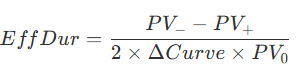
Effective Duration: For bonds with interest-rate-dependent cash flows (such as callable/putable corporate bonds, mortgage-backed securities, or floating-rate instruments), yield durations fail because the cash flows themselves alter when interest rates shift. Effective duration (or option-adjusted duration) is a curve duration statistic that measures price sensitivity to a parallel shift in the benchmark yield curve (such as the government par curve or swap curve) rather than the bond’s own yield. Using an option-pricing model, effective duration revalues the security under upward and downward benchmark curve shifts:

2. Asymmetric, Absolute, and Empirical Sensitivities

To fully capture portfolio exposure, classical parallel duration must be augmented to address asymmetrical, absolute, and credit-sensitive risk parameters:

One-Sided Durations: Because option-embedded bonds exhibit asymmetric price behavior—where price appreciation is capped when a call option is in the money, or price depreciation is limited when a put option is in the money—two-sided effective duration can be misleading. Risk managers calculate one-sided durations (specifically, one-sided up-duration and one-sided down-duration) to capture these divergent directional sensitivities in isolation.
Absolute Sensitivities (Money Duration and PVBP): Money duration (or dollar duration) measures the first-order price change in absolute currency units rather than percentages (MoneyDur=AnnModDur×PV^Full). Related to this is the price value of a basis point (PVBP / PV01 / DV01), which estimates the absolute change in the full price given a single basis-point (0.01%) yield change.
Empirical Duration: While analytical duration relies on theoretical formulas and option-pricing models, empirical duration utilizes historical price observations and regression analysis against relevant benchmark yields. For lower-rated credit sectors (such as high-yield bonds), empirical duration is systematically lower than analytical duration—and can even turn negative—because high-yield securities trade primarily based on default/recovery expectations. When Treasury rates rise, corporate credit spreads frequently compress, which dampens price sensitivity.

3. Second-Order Sensitivities: Convexity

Because the actual relationship between a bond’s price and interest rates is curved (convex) rather than straight, duration only provides a linear approximation. Convexity represents the secondary, second-order sensitivity, measuring the rate of change of duration as interest rates change (the second derivative of the price-yield function divided by price).

Similar to duration, risk managers distinguish between yield convexity and effective convexity. For straight (option-free) bonds, convexity is always positive, meaning that a more convex bond will appreciate more in price when rates fall and depreciate less in price when rates rise.

However, callable corporate bonds and MBS exhibit negative convexity (or concavity) when interest rates are low and the call/prepayment option is near the money. In this region, price appreciation is limited, causing the price-yield curve to flatten and the effective convexity to turn negative.

4. Multi-Factor Term Structure and Shaping Risks

Traditional modified and effective durations assume that interest rates of all maturities shift in parallel. In reality, yield curves are dynamic, and shifts are dominated by nonparallel changes in shape. To manage this shaping risk, modern risk measurement utilizes multi-factor models:

Key Rate Durations (Partial Durations): This approach decomposes parallel duration into a vector of sensitivities to rate changes at specific maturity segments of the benchmark curve (such as 2-year, 5-year, 10-year, or 30-year segments) while holding all other key rates constant, helping to identify steepening and flattening exposures.
Yield-Curve-Reshaping Durations: This method isolates a portfolio’s sensitivity specifically to nonparallel shifts at the short end (SEDUR) versus the long end (LEDUR) of the curve.
Level, Slope, and Curvature Durations: Utilizing Principal Component Analysis (PCA), this statistical approach explains yield curve risk through three independent movements extracted from historical covariance matrices: the first principal component represents the level factor (parallel shifts), the second is the slope/steepness factor (twists), and the third is the curvature factor (changes in the mid-maturity hump).

5. Risk Volatility and the Investment Horizon

The actual interest rate risk exposure of a bond position is a function of both its analytical price sensitivity (duration and convexity) and its yield volatility—the size and frequency of interest rate changes.

For long-term investors, the overall risk over a specific holding period is defined by the interaction between two offsetting forces: market price risk (capital losses when rates rise and prices fall) and coupon reinvestment risk (reinvesting cash flows at lower rates when interest rates drop).

The Macaulay Duration Balance Point: Macaulay duration represents the exact holding period at which reinvestment risk and market price risk perfectly offset each other under a one-time parallel yield shift.
The Duration Gap: Defined as a bond’s Macaulay duration minus the investor’s investment horizon.
- Duration Gap of Zero: The investor is immunized; coupon reinvestment changes perfectly offset capital gains or losses.
- Positive Duration Gap: The investment horizon is shorter than Macaulay duration. Market price risk dominates, and the investor is at risk of higher interest rates.
- Negative Duration Gap: The investment horizon is longer than Macaulay duration. Coupon reinvestment risk dominates, and the investor is at risk of lower interest rates.

DV01 and PVBP

1. Definitions and Core Mathematical Relationships

In fixed-income mathematics, DV01 (Dollar Value of an ’01), PV01 (Present Value or Price Value of an ’01), and PVBP (Price Value of a Basis Point) are synonymous terms representing the same fundamental risk metric. They measure the absolute currency change in the full price of a bond or portfolio for a one-basis-point (0.01% or “01”) change in interest rates.

Unlike duration, which expresses price sensitivity as a percentage change, DV01 and PVBP capture price sensitivity in absolute dollar terms.

Mathematically, the relationship is derived as follows:

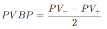
The Baseline Estimation: PVBP can be estimated by shifting the yield up and down by 1 basis point (denoted as PV₊and PV₋) and calculating the absolute price difference:

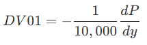
Derivative Representation: Utilizing calculus, DV01 is proportional to the first derivative of the price-rate curve (the slope of the tangent line at the current interest rate level):

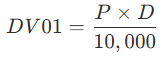
Duration Link: Because DV01 represents dollar volatility, it is mathematically linked to modified duration (D) and the bond’s full price (P):

Market Convention: On trading screens (such as Bloomberg’s Yield and Spread page), PVBP is frequently scaled up by 100 and quoted simply as “Risk”.

2. Role of DV01/PVBP in Portfolio Risk Management

While percentage-based duration is the preferred metric for long-term asset managers who invest a slowly changing pool of funds and focus on rates of return, DV01 is the standard tool for traders, market makers, and dealers:

Leveraged Financing & P&L Focus: Market makers typically borrow funds to finance their inventory and focus on absolute dollar profit and loss (P&L) rather than percentage returns. DV01 directly quantifies how many dollars are at risk in their positions.
Portfolio Additivity: One of the most powerful properties of DV01 is that the DV01 of a portfolio is completely additive. It is equal to the simple sum of the DV01s of its individual component instruments. This stands in contrast to portfolio duration, which must be calculated as a value-weighted average.

For example, a portfolio holding $10 million face amount of a century bond with a DV01 of 0.241 per 100 face amount has a position DV01 of $24,100. If that portfolio also holds a Treasury bond position with a DV01 of $20,000, the overall portfolio’s exposure to a 1-basis-point downward rate move is simply $44,100.

3. Hedging with DV01

To successfully hedge a fixed-income position, the objective is to align the absolute dollar price volatility of the hedging vehicle with the absolute dollar price volatility of the position being hedged, so that any loss on the asset is completely offset by a gain in the hedge.

Because DV01 measures this dollar price change, hedgers calculate the hedge ratio using DV01 rather than modified duration. The number of contracts or face amount of the hedging vehicle (F^B) required to hedge a target position (F^A) is given by:

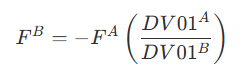
This creates a DV01-neutral position. Under a multi-factor key rate framework, a portfolio’s curve risk is managed by breaking down the total DV01 into separate “key-rate DV01s” associated with specific key maturities (e.g., 2-year, 10-year, 30-year), allowing analysts to buy or sell specific benchmark bonds to neutralize exposure at individual segments of the curve.

4. Limitations: Local Sensitivity and Convexity

DV01/PVBP is a local measure of interest rate sensitivity. It represents the slope of the tangent line to the price-yield curve at a specific point. Because the actual relationship between a bond’s price and interest rates is curved (convex), this slope is dynamic and changes continuously as rates move:

Positive Convexity: For straight, option-free bonds, as interest rates rise, the price-rate curve flattens, which means DV01 falls as interest rates increase. Conversely, DV01 rises as rates decline.
Estimation Errors: Because DV01 assumes a linear relationship, it provides highly accurate price change estimates for small movements (such as 1 basis point). However, for larger rate movements (such as 100 or 300 basis points), relying on DV01 alone systematically underestimates the new bond price. To maintain accuracy for large rate shifts, the second-order effect of convexity must be added to the duration/DV01 approximation.

5. Extended Applications: Risky DV01

The concept of DV01 is also extended to credit derivatives. In the credit default swap (CDS) market, “Risky DV01” refers to the change in the market value of a CDS contract for a single-basis-point (0.01%) change in the CDS credit spread. This metric allows credit portfolio managers to hedge and trade credit spread risk in the exact same manner that interest rate risk is managed.

Macaulay and Modified Duration

1. Macaulay Duration: The Time-Weighted Measurement of Cash Flows

Developed by Frederick Macaulay in 1938, Macaulay duration was originally designed as a proxy for the average length of time a bond’s cash flows remain outstanding. Mathematically, it is calculated as a weighted average of the time to receipt of the bond’s promised payments, where the weights represent the present value of each individual cash flow as a percentage of the bond’s full price (including accrued interest).

Macaulay duration exhibits several fundamental properties:

Zero-Coupon vs. Coupon Bonds: The Macaulay duration of a zero-coupon bond is exactly equal to its term to maturity. For a coupon bond, because some payments are received prior to maturity, its duration is always less than its time to maturity.
The Coupon and Yield Effects: Duration is inversely related to both the coupon rate and the yield-to-maturity. A lower coupon rate or a lower yield-to-maturity increases duration (and thus interest rate risk) because a larger proportion of the bond’s total value is pushed into more distant future periods.
The Passing of Time: Assuming a constant yield-to-maturity, Macaulay duration decreases smoothly as time passes during a coupon period, then jumps upward immediately after a coupon is paid, creating a distinct “saw-tooth” pattern.

2. Modified Duration: Direct Percentage Price Sensitivity

Modified duration is a direct yield duration statistic used to estimate a bond’s price responsiveness to interest rate changes. It is mathematically derived by adjusting Macaulay duration for the periodic yield:

where r is the yield per period.

Modified duration provides a linear estimate of the percentage change in a bond’s full price for a given change in its yield-to-maturity:

Because of this linear relationship, market participants frequently define modified duration as the approximate percentage price change of a bond per 100-basis-point (1.00%) change in yield. For analysts wanting a faster calculation, modified duration can be approximated directly by shocking the yield-to-maturity up and down by a small amount and calculating the resulting price changes, without first computing Macaulay duration.

3. The Horizon Balance: Reinvestment Risk vs. Market Price Risk

In the broader context of interest rate risk, long-term investors are exposed to two competing, offsetting forces:

Market Price Risk: The risk that interest rates will rise, causing the bond’s price to fall if it must be sold prior to maturity.
Coupon Reinvestment Risk: The risk that interest rates will fall, forcing the investor to reinvest periodic coupon payments at lower interest rates.

Under a one-time parallel yield curve shift, Macaulay duration represents the exact holding period (investment horizon) at which coupon reinvestment risk and market price risk perfectly offset each other. This economic relationship defines the duration gap (Macaulay duration minus the investment horizon) and shapes portfolio immunization:

Zero Duration Gap (Horizon = Duration): Reinvestment risk and price risk perfectly cancel out. The investor is immunized and assured of realizing the target yield regardless of immediate interest rate shifts.
Negative Duration Gap (Horizon > Duration): Coupon reinvestment risk dominates. The investor’s primary risk is lower rates, as the loss from reinvesting coupons at lower yields exceeds any capital gain on a potential sale.
Positive Duration Gap (Horizon < Duration): Market price risk dominates. The investor’s primary risk is higher rates, as the price drop upon sale will exceed the gains from higher coupon reinvestment rates.

4. Critical Limitations of Classical Duration Measures

While Macaulay and modified durations are essential foundation blocks of risk measurement, they carry three severe limitations:

The Parallel Shift Assumption: Both measures assume a parallel shift in the yield curve, meaning that yields across all maturities change by the same number of basis points in the same direction. In reality, yield curves are dynamic and undergo nonparallel reshaping (such as twists, steepening, or flattening), which can cause portfolios with identical parallel durations to perform vastly differently. Managing this shaping risk requires multi-factor models such as key rate durations.
The Option-Free Cash Flow Assumption: Macaulay and modified durations are yield duration statistics; they assume that cash flows are fixed and do not change when interest rates shift. For bonds with embedded options (such as callable or putable corporate bonds, or prepayable mortgage-backed securities), cash flows change dynamically as interest rates shift. To value interest-rate-sensitive cash flows, analysts must use effective duration (or curve duration), which relies on pricing models (such as binomial lattices or Monte Carlo simulations) to revalue the bond under positive and negative benchmark curve shocks.
Linearity vs. Convexity: Modified duration is a local, tangent-line linear approximation. For small interest rate shifts, it is highly accurate, but for larger rate shocks (e.g., 100 or 300 basis points), it systematically underestimates the new bond price. To maintain accuracy for large interest rate shifts, duration must be combined with convexity to provide a second-order approximation.

Effective and Key Rate Duration

Interest Rate Risk Context Traditional yield duration statistics—namely Macaulay and modified durations—have two critical limitations when measuring interest rate risk: they assume that a bond’s expected cash flows are fixed and that the yield curve only shifts in a parallel fashion. To address these unrealistic assumptions, fixed-income mathematics utilizes effective duration and key rate duration to provide a more realistic framework for managing interest rate risk.

Effective Duration (Option-Adjusted Duration) When a bond has cash flows that are contingent on future interest rates (such as callable or putable corporate bonds, or mortgage-backed securities), traditional duration metrics fail. For these securities, effective duration (or option-adjusted duration) is the only appropriate risk measure because it directly accounts for how interest rate movements alter the expected cash flows.

Mechanics of Valuation: Effective duration is a curve duration statistic that measures a bond’s price sensitivity to a parallel shift in the benchmark yield curve (such as the government par curve or swap curve) rather than changes in its own yield. The mathematical approximation is defined as:

where V₀is the current full price, V₋and V₊ and are the estimated bond prices derived from an option-pricing model (such as a binomial lattice) after shifting the benchmark curve down and up by ΔC while keeping the option-adjusted spread (OAS) constant.

Asymmetric Options Impact: The effective duration of a bond with an embedded option cannot exceed that of an otherwise identical option-free (straight) bond.
- For callable bonds, when rates fall, the call option moves into the money, limiting the bond’s price appreciation and shortening its effective duration.
- For putable bonds, when rates rise, the put option moves into the money, limiting price depreciation and shortening its effective duration. When an option is deep in the money, the effective duration will compress to match that of a straight bond maturing on the first exercise date.

Key Rate Duration (Partial Duration) Even for option-free bonds, parallel shifts in the yield curve are rare; the shape of the yield curve shifts continually due to changes in level, steepness, and curvature. Key rate duration (or partial duration) is designed to measure and manage this shaping risk by isolating how a bond’s price responds to a change in the interest rate at a single maturity segment of the benchmark curve while keeping all other segment rates constant.

Mechanics of Shifts: To calculate key rate durations, analysts select a set of key maturities (often aligned with the maturities of liquid on-the-run Treasury benchmark bonds, such as 2-year, 5-year, 10-year, and 30-year segments). When a key rate is shifted, par rate changes are assumed to decline linearly to zero at the adjacent key rates. The sum of all key rate durations of a portfolio is mathematically equal (or very nearly equal) to the portfolio’s total parallel effective duration.
Cash Flow Distribution on Option-Free Bonds:
- For a straight bond trading at par, the maturity-matched key rate is the only rate that affects its value. Shifting other key rate segments has no impact because the par rates at other points do not alter the terminal principal discounting.
- For a straight bond not trading at par (discount or premium), other rates have minor impacts, but the maturity-matched rate still heavily dominates because the largest cash flow (principal plus coupon) occurs at maturity.
- For zero-coupon or very low-coupon bonds, shifting shorter-term key rates can occasionally result in negative key rate durations due to the mathematical relationship between par rate shifts and the derived spot discount rates.

The Intersection: Key Rate Durations for Option-Embedded Bonds For bonds with embedded options, key rate durations do not just depend on the final maturity date; they are highly sensitive to both the time to maturity and the time to option exercise. The dominant key rate exposure will dynamically shift depending on the likelihood of the option being exercised:

Callable Bond Dynamics: Consider a 30-year bond callable in 10 years. If the coupon is low (e.g., 2%), the call option is out of the money and unlikely to be exercised, causing the bond to behave like a 30-year straight bond where interest rate risk is concentrated in the 30-year key rate. However, as the coupon rate increases, the likelihood of a call increases, shortening the total duration and shifting the dominant pricing sensitivity from the 30-year key rate to the 10-year key rate. At a very high coupon (e.g., 10%), the bond is virtually certain to be called, and its key rate duration profile behaves entirely like a 10-year straight bond.
Putable Bond Dynamics: Conversely, for a 30-year bond putable in 10 years, a high coupon means it is unlikely to be put, concentrating risk in the 30-year key rate. If the coupon is low, it is highly likely to be put, compressing its interest rate risk into the 10-year key rate segment.

Approximate and Effective Convexity

The Price-Rate Curve and the Need for Convexity

While modified and effective durations provide a first-order linear approximation of a bond’s price sensitivity to interest rate changes, they assume a straight-line relationship. In reality, the actual relationship between a bond’s price and interest rates is curved, or convex.

Because of this curvature, a duration-only price approximation systematically underestimates the actual bond price at a new yield level. For small interest rate shifts, this underestimation is negligible; however, for larger rate shocks (such as 100 or 300 basis points), the discrepancy becomes substantial.

To improve the accuracy of the estimate, fixed-income mathematics utilizes a second-order approximation derived from a Taylor series expansion, which combines duration and convexity:

1. Approximate Convexity

Approximate convexity is a yield-based risk statistic used for option-free bonds. It is calculated by assuming that a bond’s scheduled cash flows remain constant and do not change when interest rates shift.

Mathematical Formulation

To approximate the convexity of a bond numerically, an analyst shifts the bond’s yield-to-maturity up and down by a small, equal interval (ΔYield), revalues the bond at those shifted yields, and applies the following formula:

where:

PV0 is the initial full price of the bond.
PV+ is the estimated full price of the bond if the yield is increased by ΔYield.
PV− is the estimated full price of the bond if the yield is decreased by ΔYield.

For any straight (option-free) bond, the calculated convexity measure is always positive. This means that the convexity adjustment term, 1/2 × Convexity × (ΔYield)² , will always add a positive increment to the estimated price change, regardless of whether interest rates increase or decrease.

2. Effective Convexity

Yield-based approximate convexity fails when a security features interest-rate-dependent cash flows—such as corporate bonds with embedded call or put options, and mortgage-backed securities (MBS) subject to prepayment risk. For these instruments, a change in interest rates dynamically alters the expected timing and magnitude of the cash flows themselves.

Effective convexity (or option-adjusted convexity) resolves this by using an option-pricing model (such as a calibrated binomial interest rate lattice or a Monte Carlo simulation) to allow the cash flows to change as yields change.

Mathematical Formulation and Key Difference

Effective convexity uses a functionally identical approximation formula, but with one critical distinction in the denominator:

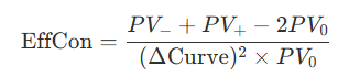
In approximate convexity, the denominator is based on the change in the bond’s own yield-to-maturity (ΔYield).
In effective convexity, the denominator is based on a parallel shift in the entire benchmark yield curve (ΔCurve), such as the government par curve or swap curve, while keeping the bond’s option-adjusted spread (OAS) constant.

3. Asymmetric Option Behavior and Negative Convexity

While straight option-free bonds always exhibit positive convexity, the presence of embedded options introduces dramatic asymmetries:

Callable Bonds (Negative Convexity)

When interest rates are high relative to a callable bond’s coupon rate, the call option is out of the money and unlikely to be exercised. Under these conditions, the callable bond behaves similarly to a straight bond, exhibiting positive convexity.

However, as interest rates decline, the likelihood of the issuer exercising the call option to refinance their debt increases. The potential price appreciation of the bond is capped near the call price (price compression). At this point, the pricing relationship reaches an inflection point, and the effective convexity turns negative (concave).

Under negative convexity, the absolute value of the price appreciation when rates fall is less than the price depreciation when rates rise:

Interest Rate Change	Straight Bond Price Response	Callable Bond Price Response (Near the Money)
Rates Fall (−ΔYield)	Large Price Increase	Limited Price Increase (Capped)
Rates Rise (+ΔYield)	Moderate Price Decrease	Full Price Decrease

Putable Bonds (Enhanced Positive Convexity)

Conversely, an embedded put option protects the investor. When interest rates rise, the put option moves into the money, allowing the bondholder to sell the bond back to the issuer at par. This floor prevents the bond price from falling below the put price, meaning putable bonds maintain positive convexity at all yield levels. When rates rise, their price depreciation is limited, causing the pricing curve to flatten and effective convexity to remain highly favorable.

4. Portfolio Management and the “Cost of Convexity”

In portfolio construction and Asset-Liability Management (ALM), convexity is a critical factor:

Portfolio Additivity: The convexity of a portfolio is equal to the weighted average of the convexities of its individual holdings, where the weights are determined by each bond’s market value as a percentage of the total portfolio value.
The Volatility Play: Because positive convexity improves price performance when rates move in either direction, a more convex bond will always outperform an otherwise identical, less convex bond in both bull and bear markets. Because of this structural advantage, investors must “pay up” for positive convexity. This is reflected in the market offering lower yields for highly convex portfolios (known as the cost of convexity).
Barbell vs. Bullet Portfolios: Among portfolios matching the same target duration, a barbell portfolio (which disperses cash flows far into the short and long ends of the curve) exhibits much larger convexity than a bullet portfolio (which concentrates cash flows around the target maturity date). Because convexity scales quadratically with maturity while duration scales roughly linearly, the long-term bonds in the barbell dominate the portfolio’s overall convexity.
The ALM Convexity Mismatch: In a pension fund setting, matching the duration of assets and liabilities is not enough. If liabilities possess greater convexity than the assets (a negative convexity position), the pension fund faces net losses if rates move significantly in either direction. Portfolio managers must balance the extra yield earned from a less-convex bullet portfolio against the superior risk protection and reduced rebalancing costs offered by a highly convex barbell portfolio.

Credit and Liquidity Risk

Credit and Liquidity Risk in the Larger Context of Risk Measurement

In modern fixed-income portfolio management, the evaluation of risk has undergone a dramatic transformation. Before the 1980s, in a more stable interest rate environment, risk measurement was dominated by simple buy-and-hold analytics: credit risk was gauged primarily by credit agency ratings, and interest rate risk was approximated using the yield-to-maturity or yield-to-call. Today, fixed-income portfolios are actively and globally traded, which has elevated the necessity of integrating sophisticated statistical, mathematical, and data-science techniques to quantify credit risk, liquidity risk, and multi-factor curve exposures in a unified risk-measurement framework.

1. Credit Risk: Decomposing Default and Spread Risks

Credit risk is defined as the risk of financial loss resulting from a borrower failing to make full and timely payments of interest or principal. Risk managers divide credit risk into two primary components: credit default risk and credit spread risk.

Credit Default Risk and Expected Loss

Default risk is the probability that an obligor fails to meet its contractual debt obligations. In quantitative risk measurement, this is analyzed through three core metrics: Exposure at Default (EAD), Loss Given Default (LGD) (which is ), and Expected Loss (EL):

Expected Loss=Default Probability (PD)×Loss Given Default (LGD)

Because holders of defaulted bonds typically recover some value through liquidation or reorganization, analyzing potential LGD is critical—especially for high-yield or distressed debt where default probabilities are elevated.

To model default probabilities (PD) on corporate debt, analysts employ two dominant quantitative frameworks:

Structural Models (Firm-Value Models): Originating from Robert Merton’s 1974 work, these models view default as an option-type event. Equity is modeled as a European call option on the company’s underlying assets, while risky debt is valued as a default-free bond minus a European put option on the firm’s assets. Because firm asset values are not directly observable, structural models must be estimated implicitly by calibrating option formulas to publicly traded equity prices.
Reduced-Form Models: These models (such as Jarrow-Turnbull and Duffie-Singleton) do not look inside the firm’s balance sheet. Instead, they model default directly as a random surprise event governed by a default intensity process (or Cox/Poisson process). This allows default probabilities to vary dynamically with macroeconomic variables and the business cycle. Crucially, reduced-form parameters can be estimated historically using logistic regressions on public company default databases.

The Present Value of Expected Loss (PVEL)

While Expected Loss is an actuarial measure, risk measurement in a trading or marking-to-market context relies on the Present Value of Expected Loss (PVEL). PVEL represents the maximum price an investor would pay to a default-free third party to completely eliminate a bond’s credit risk. To capture risk premium and the time value of money, PVEL adjusts the actual probabilities of default to risk-neutral probabilities (discounting the expected losses at the risk-free rate).

Credit Spread Risk and Volatility Metrics

Spread risk represents the potential price decline of a bond due to a widening of its credit spread over the risk-free benchmark curve. Traditional spread measurement utilizes credit spread duration, which approximates the percentage price change of a bond for a 100-basis-point parallel shift in its spread. However, modern risk systems utilize more advanced spread risk metrics:

Duration Times Spread (DTS): Developed as the market standard for credit volatility, DTS is the product of credit spread duration and the credit spread itself. DTS is mathematically superior to spread duration because empirical credit spread changes are proportional to the absolute level of the spread (i.e., bonds with wider spreads experience larger absolute spread movements).
Hazard-Adjusted Duration (HAD): Conventional duration assumes that cash flows are fixed and paid on schedule. For highly distressed bonds, HAD calculates duration based on the expected timing of cash flows under risk-neutral default and recovery assumptions, resulting in significantly shorter and more realistic duration estimates.
Risky DV01: Used primarily in credit derivatives (CDS) and basis trading, Risky DV01 measures the absolute dollar change in the contract’s value for a single-basis-point change in the CDS credit spread.

2. Liquidity Risk: Transaction Costs and Price Impact

Liquidity risk is the threat of financial loss due to transaction costs when executing a trade, or the inability to execute trades quickly at a price close to the prevailing market level. Measuring and modeling liquidity risk in the fixed-income market is exceptionally challenging because most bonds trade over-the-counter (OTC) through dealer networks, and the vast majority of individual issues trade very infrequently.

The Dimensions of Liquidity

According to IMF and Basel frameworks, liquidity risk possesses several key dimensions:

Tightness: The cost of trading, typically measured by the bid-ask spread.
Immediacy: The speed with which an order can be executed.
Depth and Breadth: The existence of abundant orders of varying sizes that can be executed with minimal impact on prices.
Resiliency: The speed at which new orders arrive to correct temporary market price imbalances.

Transaction costs are split into explicit costs (fees, commissions) and implicit costs. The primary implicit cost is market impact cost—the price concession required to induce dealers to commit capital to a transaction. This can be decomposed into a temporary market impact (due to immediate inventory imbalances) and a permanent market impact (reflecting the information content of the trade as the market adjusts to potential overvaluation or undervaluation).

Quantitative Liquidity Measurement

To monitor liquidity risk, risk managers classify liquidity metrics into three categories:

Raw Data Measures: Quantity-based metrics (trades per day, number of quoting sources) and price-based metrics (observed bid-ask spreads).
Adjusted Single-Datum Measures: Refined price-based indicators, including Roll’s price reversal measure (an implicit spread estimated from the negative serial autocorrelation of observed transaction prices), the Amihud index (measuring the price impact per unit of volume), and the lambda measure.
Liquidity Scores: Statistical scores designed to capture multiple dimensions of liquidity simultaneously. The most prominent is the Barclays Liquidity Cost Score (LCS), which measures the percentage cost of a standard institutional-sized round-trip transaction. For spread-quoted bonds, the LCS is calculated as:

LCS=(bid spread−ask spread)×OASD

where OASD is the option-adjusted spread duration. For bonds without real-time quotes, a cross-sectional multiple linear regression estimates the LCS by relating observable bond attributes (such as age, issue size, monthly volume, credit rating, and DTS) to the scores of quoted bonds.

3. Integration into the Larger Context of Risk Measurement

Credit and liquidity risks do not operate in isolation; they are deeply intertwined with interest rate risk and are integrated into comprehensive risk-measurement systems through modern portfolio techniques.

Non-Normal Returns and Downside Risk Measures

Because option-embedded bonds, prepayable mortgage-backed securities, and default-prone credit assets exhibit highly skewed, fat-tailed return distributions, standard portfolio metrics like standard deviation and variance (which assume normality) are insufficient. Portfolio managers supplement these with downside and shortfall risk measures:

Shortfall Risk: The probability that a portfolio’s return will fall below a specified minimum acceptable return.
Value at Risk (VaR): A probability-based estimate of the minimum dollar loss expected to be exceeded over a specified horizon at a given confidence level (e.g., 95% or 99%).
Conditional Value at Risk (CVaR) / Expected Shortfall: Measures the average loss in the worst-case outcomes that lie beyond the VaR threshold.

Tracking Error and Factor Models

In passive indexation or risk-budgeted active portfolio management, risk is measured using tracking error (tracking risk)—the standard deviation of the portfolio’s active returns relative to a benchmark index.

In a multi-factor risk model (such as the Axioma, Amundi, or Lehman models), the portfolio’s forward-looking, predictive tracking error is decomposed using a factor covariance matrix. This allows risk managers to isolate the exact contribution of each underlying risk category to the total portfolio risk:

Yield-Curve (Rates) Risk: Sensitivity to changes in the level, slope, and curvature of the benchmark sovereign term structure.
Swap-Spread Risk: Exposure to movements in the swap curve relative to government benchmarks.
Corporate Spread Risk: The credit spread risk, typically measured using active DTS mismatches.
Securitized Spread Risk: Exposure to prepayment, refinancing, and turnover risks in mortgage-backed and asset-backed portfolios.
Volatility Risk: Sensitivity to implied volatility (vega) changes in swaptions or options embedded within corporate and structured debt.
Specific (Idiosyncratic) Risk: The residual credit and liquidity risk specific to an individual issuer or issue that cannot be explained by systematic factors.

By modeling the correlations and covariances among these risk factors, risk measurement systems prevent the dangerous assumption that risk factors move independently, capturing the real-world reality where a systemic financial crisis simultaneously triggers lower benchmark yields (flight to quality), widening credit spreads, and a severe contraction in market liquidity.

Default and Recovery Rates

In the broader analysis of credit and liquidity risk, default is contractually defined as a failure by a borrower to meet its debt obligations, such as any missed or delayed disbursement of interest and/or principal . When an issuer defaults, the actual financial loss incurred by the investor is equal to the outstanding obligation at default minus any recovery amount received via foreclosure, liquidation, or restructuring .

1. Default Rate Metrics

To track historical credit performance, analysts measure defaults across portfolios using two primary metrics:

Issuer Default Rate: This treats the individual borrowing entity as the single unit of observation, calculating the percentage of defaulting issuers relative to the total number of active issuers at the start of the year, completely ignoring the dollar size of the liabilities .
Dollar Default Rate: This defines the default rate as the total par value of all defaulted bonds in a calendar year divided by the total par value of all outstanding bonds during that year, reflecting the absolute financial scale of credit impairment .

2. Recovery Rates and Loss Given Default (LGD)

In portfolio management, default rates alone do not dictate overall returns; a portfolio with defaults can still outperform Treasuries if its yield spreads are high enough to offset the experienced credit losses . Therefore, modern risk systems decompose credit risk into Exposure at Default (EAD)—the outstanding obligation when default occurs—and Loss Given Default (LGD)—the fraction of EAD that is ultimately not recovered .

The Analytical Link: The recovery rate is mathematically defined as 1−LGD .
The Measurement Challenge: Measuring actual recoveries is complex because restructuring settlements frequently consist of a non-standard mix of cash, new debt, and equity . To resolve this, rating agencies like Moody’s utilize the trading price of the bond immediately after default divided by its par value as a market-implied proxy for the recovery rate .
Historical Averages (1983–2020): For senior unsecured corporate debt, investment-grade issues experienced an average five-year default rate of 0.9% and an average recovery rate of 44.5% (yielding an average credit loss of 0.5%) . Speculative-grade issues had an average default rate of 19.6% and a recovery rate of 38.3% (resulting in an average credit loss of 12.2%) .
Market Convention: In standard pricing and credit derivative modeling, market participants widely assume a baseline recovery rate of 40% for senior unsecured corporate debt .

3. Capital Seniority and the Priority of Claims

Recovery rates are heavily dictated by an issuer’s capital structure and the contractually defined priority of claims in a bankruptcy proceeding:

Secured vs. Unsecured claims: Secured debt (such as first mortgage or first lien debt) has a direct, senior claim on specific pledged collateral . Unsecured debt (debentures) ranks below secured claims and relies on the general, unpledged assets and cash flows of the issuer .
Liquidation vs. Reorganization: In a formal liquidation of corporate assets, the absolute priority rule—which guarantees that senior creditors are paid 100% in full before junior creditors receive any recovery—generally holds true . In corporate reorganizations (such as US Chapter 11), however, strict absolute priority is frequently compromised . Because protracted court battles consume the remaining cash value of the estate, senior creditors often negotiate compromises with subordinated holders and shareholders to allow the firm to emerge quickly as a going concern .
Regulatory Jurisdictions: Bankruptcy laws differ significantly by geography; the legal framework in the United States is structurally biased toward reorganization and company recovery, whereas the United Kingdom is biased toward liquidation and maximizing immediate value for senior bank lenders .

4. Quantitative and Statistical Modeling of Credit Risk

To price credit assets and calculate expected losses, analysts rely on two primary quantitative modeling frameworks:

Structural Models (Firm-Value Models): Pioneered by Robert Merton, these models view default as occurring when the total value of the firm’s assets falls below the face value of its liabilities at maturity . Equity is treated as a European call option on the company’s assets, meaning that default probability and recovery rates are mathematically bound to the assumed balance sheet structure and the unobservable volatility of firm assets .
Reduced-Form Models: These bypass the balance sheet structure, modeling default directly as a random surprise event governed by a default intensity process (hazard rate) that depends on a vector of macroeconomic state variables . LGD is also modeled as state-dependent, allowing default probabilities and loss severities to expand during economic recessions and contract during economic expansions .
Hazard Rate and Machine Learning Estimation: Analysts historically estimate these models using logistic regressions (hazard rate estimation) on large public databases, linking binary default outcomes to macroeconomic indicators (e.g., unemployment rates) and company-specific financials (e.g., leverage and cash-to-assets) . Furthermore, machine learning algorithms—including regression trees, bagging, and support-vector regressions (SVR)—are increasingly deployed to forecast corporate bond recovery rates out of sample, consistently outperforming traditional linear models .

5. The Dynamic Intersection with Liquidity Risk

Default risk and trading illiquidity are highly correlated and compound one another in times of financial distress:

Exacerbated Distress: Traditional credit models historically assumed credit default risk was idiosyncratic and could be diversified away . In reality, when a bond’s credit quality deteriorates, the direct default loss is severely exacerbated by illiquidity . Dealers withdraw balance sheet capital, bid-ask spreads widen, and trading volume evaporates .
Execution Impediments: This illiquidity makes it extremely difficult for a manager to execute “credit defense” trades to liquidate deteriorating holdings before an actual default occurs, often forcing them to hold the security or accept fire-sale valuations .
Financing (Funding) Liquidity Risk: In relative-value arbitrage trades like the CDS-bond basis (which exploits price discrepancies between a corporate bond’s spread and its CDS premium), cash flows are theoretically matched to maturity . However, because long-term corporate repurchase agreements (repo) do not exist, traders are exposed to acute short-term financing risk . If market liquidity contracts or the issuer’s credit degrades, overnight repo lenders can instantly raise haircuts (as occurred to MF Global in 2011, where haircuts on European sovereign repo surged from 3% to 80%) or refuse to roll the financing, forcing a catastrophic unwinding of the position at distressed prices .

Credit Spread Duration

Credit spread duration (or simply spread duration) measures a security or portfolio’s price sensitivity to changes in the credit spread—the excess yield over the government risk-free benchmark curve required by the market to take on credit risk. While standard duration measures (such as modified or effective duration) quantify sensitivity specifically to changes in benchmark risk-free Treasury rates, spread duration isolates price sensitivity to any factor that causes the yield spread itself to shift.

In practical terms, it is interpreted as the approximate percentage change in the price of a bond for a 100-basis-point (1.00%) change in the credit spread. For example, a bond with a spread duration of 2.8 will see its price change by approximately 2.8% for every 100-basis-point movement in its credit spread.

1. Fixed-Rate Bonds versus Floating-Rate Notes (Floaters)

The structural mechanics of spread duration are highly dependent on the bond’s coupon design:

Fixed-Rate Bonds: Spread duration represents the sensitivity of the bond’s price to changes in its yield spread relative to Treasuries. For a portfolio containing both Treasury and non-Treasury securities, the overall portfolio spread duration will differ from its interest rate duration because the spread duration of Treasury securities is contractually zero.
Floating-Rate Notes (FRNs): For floaters, spread duration measures price sensitivity specifically to changes in the quoted margin or discount margin required by the market, assuming the underlying benchmark reference rate (such as SOFR or Euribor) remains unchanged.

2. Disentangling Credit and Optionality Exposure

The yield spread of a corporate bond may be driven by multiple distinct risk factors. Analysts attempt to qualify and isolate these individual exposures:

Credit Spread Duration: This label is specifically applied when the spread sensitivity is driven primarily by the issuer’s default and credit migration risks.
Option-Adjusted Spread (OAS) Duration: For bonds with embedded options (such as callable or putable corporate issues), the expected cash flows are interest-rate sensitive. Analysts utilize option-pricing models to separate the spread duration arising from changes in the clean credit spread from the spread changes caused by the changing value of the embedded call or put option.

3. Credit Spread Risk and Mathematical Equivalence

Credit spread risk is the risk of financial loss resulting from changes in the credit spreads used to mark-to-market a debt portfolio. For a traditional, option-free fixed-rate bond, the same analytical duration and convexity statistics apply to a change in the benchmark yield as to a change in the spread.

From an analytical standpoint, this means that “interest rate duration,” “credit duration,” and “liquidity duration” are mathematically the exact same number. The bond will appreciate or depreciate in value by the same estimated amount regardless of whether the yield-to-maturity change originates in macroeconomic benchmark rates or in microeconomic spreads.

4. The Transition to Duration Times Spread (DTS)

While credit spread duration is a valuable metric, the market standard for quantifying portfolio credit volatility is Duration Times Spread (DTS), developed jointly by researchers at Robeco and Lehman Brothers. DTS is the mathematical product of a bond’s credit spread duration (D_spread) and its credit spread (s):

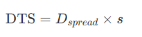
DTS is a superior risk metric because empirical evidence from bond markets demonstrates that credit spread changes are proportional to the absolute level of the credit spread. This means that bonds with wider spreads are highly likely to experience larger absolute spread changes than bonds trading at tighter spreads. Mathematically, the percentage price change due to a spread shift is expressed as:

This equation demonstrates that percentage price volatility is driven by the percentage change in the spread (Δs/s) scaled by the DTS.

However, risk managers must recognize a critical boundary of DTS: it only measures the credit risk associated with spread volatility, not default risk. For example, a lower-rated high-yield bond with a short spread duration can have the exact same DTS as a higher-rated investment-grade bond with a long spread duration. While their expected spread-driven mark-to-market price volatilities are identical under this metric, the lower-rated bond carries substantially higher credit default risk.

5. Exacerbation by Liquidity Risk

In the broader context of risk measurement, spread duration and credit risk do not operate in isolation from liquidity. Corporate and structured markets can experience periods of severe distress, such as when market makers or dealers withdraw capital commitments. When an issuer or sector becomes distressed, the direct capital losses from credit spread widening (captured by spread duration and DTS) are severely compounded and exacerbated by market illiquidity. Bid-ask spreads widen significantly, and trading volume evaporates, preventing managers from executing timely “credit-defense” trades to liquidate deteriorating assets before an actual default occurs.

Credit Ratings

In fixed-income markets, credit ratings serve as an essential mechanism for evaluating and pricing credit risk, but their application also has profound, systemic impacts on market liquidity. The relationship between credit ratings and credit and liquidity risks is defined by several structural, analytical, and behavioral dynamics.

1. The Nature of Credit Ratings: Ordinal vs. Issue Ratings

Credit ratings, provided by major credit rating agencies like Moody’s, Standard & Poor’s (S&P), and Fitch, are formal opinions regarding the credit default risk of a debt issuer or a specific debt issue.

Ordinal Rankings: Credit ratings are ordinal rankings rather than cardinal rankings. They order borrowers and debt issues from highest to lowest risk of default, but they do not provide a precise mathematical estimate of a bond’s probability of default, nor do they signify that a specific rating step is exactly twice as risky as another.
Issuer vs. Issue Ratings: An issuer credit rating measures an obligor’s overall creditworthiness to meet its financial obligations, typically represented by its senior unsecured rating. An issue credit rating applies to a specific financial obligation, taking into account the priority of payment and seniority ranking.
The Notching Process: To distinguish between the risk profiles of different debt instruments from the same issuer, rating agencies use a process called notching. Issue ratings are moved up or down from the issuer’s corporate credit rating to reflect factors such as collateral backing, seniority ranking, and structural subordination. S&P’s notching guidelines dictate that as default risk increases, the potential loss given default (LGD) is weighted more heavily, meaning subordinated debt is notched further below the issuer rating for speculative-grade credits (up to two notches) than for investment-grade credits (usually one notch).

2. Credit Risk and the “Stability-Accuracy” Tension

For long-term debt, a credit rating represents a forward-looking assessment of both the probability of default and the relative loss severity should a default occur. In evaluating this credit risk, rating agencies must navigate a fundamental tension between ratings stability and ratings accuracy:

The Preference for Stability: Rating agencies tend to keep ratings stable across the business cycle to prevent excessive price volatility in the debt markets.
The Accuracy Sacrifice: Because ratings are designed to change infrequently, the relationship between a static rating and its actual default probability is non-constant over time. For example, although the rating of a speculative issuer remains constant at CCC, the actual annual default rate for S&P’s CCC-rated pool varies dramatically with the macroeconomic environment—ranging from 0% in the healthy economy of 1981 to 48.68% during the 2009 recession.

3. Limitations and Risks of Relying on Credit Ratings

Although ratings provide a simple, comparable statistic to summarize complex credit analysis, relying solely on them exposes investors to significant credit-related risks:

Lagging the Market: Ratings tend to lag the market’s pricing of credit risk. Credit spreads and bond prices consistently adjust on a daily basis in response to changing creditworthiness, whereas rating agencies change their ratings or outlooks much more slowly (as historically demonstrated by Ford Motor Company’s bond prices during the financial crisis).
Ratings Migration: Credit ratings are not static; they migrate over time, with lower-rated debt exhibiting much higher instability. Transition tables show that while higher-rated credits are highly stable, single-B rated credits only maintain their rating over a three-year period about 40% of the time.
Unmodeled Risks: Ratings struggle to capture unpredictable or low-probability/high-severity risks, such as litigation risk, environmental liabilities, or sudden debt-financed leveraged buyouts (LBOs) and stock buybacks. They also cannot account for accounting fraud (e.g., Enron, WorldCom, and Parmalat).
Expected Loss Mismatch: Two issuers with the same credit rating (representing a comparable probability of default) may trade at very different prices because the market evaluates expected loss (the product of default probability and loss severity). A bond with a higher expected recovery rate will trade at a higher price than a similarly rated bond with a lower recovery rate.
The Issuer-Pays Conflict: The prevailing issuer-pays model, where the borrowing entity pays the credit agency to rate its debt, creates an inherent conflict of interest that can lead to overly optimistic or distorted ratings.

4. The Intersection of Credit Ratings and Liquidity Risk

Credit ratings are a primary driver of both an individual asset’s trading liquidity and systemic market liquidity risk:

High Ratings and HQLAs: In liquidity frameworks (such as Basel III), an asset’s liquidity is directly tied to its credit standing. Low-risk assets with high credit standing and a low degree of subordination tend to have much higher liquidity.
The “Fallen Angel” Downgrade Shock: The boundary between investment-grade (Baa3/BBB- or higher) and speculative-grade/high-yield (Bal/BB+ or lower) ratings is structurally critical. Regulated financial intermediaries (such as banks and life insurance companies) and certain institutional portfolios operate under strict statutory or investment policy statement (IPS) guidelines that restrict or prohibit the holding of speculative-grade debt.
Forced Selling and Bid-Ask Spread Widening: When an issuer loses its investment-grade status and is downgraded to speculative-grade, institutional investors are often forced to immediately liquidate their holdings. Because the high-yield corporate bond market is structurally much less liquid than the investment-grade market, dumping large volumes of a “fallen angel” onto a decentralized, over-the-counter (OTC) dealer market—especially during a crisis when dealers are reluctant to commit balance-sheet capital—results in a severe decline in market liquidity. Bid-ask spreads widen dramatically, and investors are forced to realize massive capital losses at the worst possible time.
Liquidity Scoring Models: This dynamic is reflected in quantitative liquidity modeling. In the Barclays Liquidity Cost Score (LCS), which measures the percentage cost of a standard institutional round-trip transaction, the credit rating is a universally significant explanatory variable alongside Duration Times Spread (DTS). Similarly, Amundi’s Liquidity Score (LS) model confirms that investment-grade bonds are structurally more liquid than high-yield bonds, and that higher credit ratings are directly correlated with lower transaction costs.

Liquidity Metrics and Transaction Costs

Liquidity in fixed-income markets is a multi-dimensional concept that generally refers to the ability to execute large transactions quickly with limited price impact, low transaction costs, and immediate execution. Historically, the Bank for International Settlements (BIS) has defined market liquidity as “the ability to rapidly execute large financial transactions with a limited price impact”. In the context of risk management, liquidity is a critical factor because when a bond becomes distressed, the direct credit loss is almost always severely exacerbated by illiquidity.

To quantify this risk and manage portfolios under both normal and stressed market conditions, analysts rely on a combination of transaction cost analysis and quantitative liquidity metrics.

1. The Dimensions and Categories of Transaction Costs

Liquidity and transaction costs are highly interrelated; a highly liquid market is one where large trades can be completed immediately without realizing high transaction costs. Fixed-income transaction costs are broadly categorized into fixed versus variable costs and explicit versus implicit costs:

Fixed costs are independent of trade size and market conditions, while variable costs depend on these factors and can be optimized by managers.
Explicit (Observable) costs are known upfront. In over-the-counter (OTC) bond markets, these are primarily bid-ask spreads—the difference between the price at which a dealer is willing to buy (bid) and sell (ask) a security. The spread represents the immediate price charged by dealers for supplying immediacy and short-term price stability in the face of order imbalances.
Implicit (Nonobservable) costs are not known prior to a trade and typically constitute the largest component of total transaction costs. These include:
- Investment Delay Cost: The price change (possibly market-adjusted) that occurs between the time a portfolio manager decides to trade and when the trade is executed.
- Opportunity Cost: The cost of failing to execute a trade, defined as the performance difference between the desired investment and the actual investment after transaction costs.
- Market (Price) Impact Cost: The difference between the actual execution price and the estimated price that would have prevailed had the trade not occurred. This is further decomposed into:
  - Temporary impact: Transitory price movements resulting from the liquidity concession required to induce a market maker to absorb inventory imbalances.
  - Permanent impact: Persistent price changes that occur as the market adjusts to the perceived information content of the trade (e.g., a sell order signaling overvaluation, or a buy order signaling undervaluation).
- Crowding Cost: The adverse price impact and elevated transaction costs that occur when multiple asset managers employ identical active strategies and simultaneously attempt to execute trades on the same bond.

2. Challenges in Measuring Bond Liquidity

Measuring and modeling fixed-income liquidity risk is significantly more challenging than in equity markets. Because the vast majority of bonds trade over-the-counter rather than on centralized exchanges, transaction details are opaque. Key structural challenges include:

Infrequent Trading: On any given day, only a tiny fraction of the outstanding bond universe actually trades. However, a lack of active trading does not automatically mean a bond is illiquid; highly rated structured bonds held by buy-and-hold institutions can be easily liquidated at fair prices if put out for bid.
Indicative vs. Transaction Prices: Many market data sources rely on indicative quotes (dealer bids/offers) rather than actual transaction prices. Indicative quotes are subject to change, but because they are more widely available than actual trade data, they can serve as valuable forward-looking proxies.
TRACE Limitations: In the United States, transaction data is reported via the Trade Reporting and Compliance Engine (TRACE). However, TRACE imposes a cap on the reported size of very large trades, which effectively masks the true price impact of the massive transactions most critical to portfolio managers.

3. Quantitative Bond Liquidity Metrics and Scores

To monitor and manage liquidity risk, the fixed-income industry categorizes liquidity measures into three distinct types:

A. Raw Data Measures

These are single, unadjusted measures based on market data. They can be quantity-based (intensity of trading, such as average daily volume [ADV], turnover, or the number of trades/quotes per day) or price-based (observed bid-ask spreads).

B. Adjusted Single-Datum Measures

These refine raw data to isolate specific aspects of liquidity:

Roll’s Price Reversal Measure: An implicit spread measure computed from the serial autocorrelation of observed transaction prices, exploiting the reality that prices continuously bounce between the bid and ask as buy and sell orders arrive randomly.
The Amihud Index: Calculated by dividing the average absolute price change between consecutive trades by the trading volume. By measuring the price impact per unit of volume, it directly captures the market’s depth and resilience.
The Lambda Measure: Employs econometric regression models to map the relationship between trade returns and signed trading volumes on a given day.
Zero-Return Days: The proportion of days in a given month during which a bond does not trade; a higher number of idle days indicates lower liquidity.

C. Liquidity Scores

Because no single metric can capture all dimensions of liquidity, data vendors and asset managers use multivariate statistical models to compile comprehensive scores:

Barclays’ Liquidity Cost Score (LCS): Introduced in 2009, the LCS represents the percentage cost of executing a standard institutional-sized round-trip transaction. For spread-quoted bonds, it is calculated as LCS = (bid spread – ask spread) × Option-Adjusted Spread Duration (OASD). For nonquoted bonds, a cross-sectional multiple linear regression estimates the LCS using observable bond attributes. Empirical tests show that Duration Times Spread (DTS) is universally the most significant explanatory variable in these regressions, while trading volume is among the least.
Ben Slimane-de Jong Liquidity Score (Amundi LS): This scoring model replaces all observed spreads with modeled equivalents via multiple regression analysis to bypass the issue of unreliable quotes. The model’s findings align with market expectations:
- Sovereign Treasuries are structurally more liquid than non-Treasuries, and investment-grade corporate bonds are far more liquid than high-yield bonds.
- Inflation-linked, subordinated, and zero-coupon bonds are relatively illiquid.
- Issue size is the most dominant determinant of liquidity, followed by issuer size.
- A higher coupon, a higher credit rating, a younger bond age, and “on-the-run” benchmark status are all directly correlated with better liquidity and lower transaction costs.

4. The Broader Context of Credit and Liquidity Risk

Credit risk and liquidity risk do not operate in isolation; they are deeply intertwined, particularly during periods of market distress.

Regulatory Frameworks and HQLA

Under the global Basel III banking regulations, banks must maintain a Liquidity Coverage Ratio (LCR), requiring them to hold sufficient High-Quality Liquid Assets (HQLAs) to survive a 30-day stress scenario. HQLAs are defined as assets that can be easily and immediately converted into cash at little or no loss of value. To qualify, assets must exhibit low credit risk, high credit standing, a low degree of subordination, low duration, and simple, standardized structures—factors that naturally promote agreed-upon valuations and deep trading markets.

Dealer Capital and Systemic Fragility

Traditionally, dealers supplied market liquidity by committing their own balance-sheet capital to buy and hold inventory, absorbing the execution and market risks of large client orders. However, post-crisis regulatory overhauls (such as capital requirements, leverage ratios, and the Volcker Rule) have severely restricted banks from trading for their own accounts. As banking entities have withdrawn capital commitments, primary dealers hold much smaller net inventories of corporate bonds relative to the total volume outstanding. While the growth of Principal Trading Firms (PTFs) and electronic platforms has made liquidity plentiful for small trades, liquidity for large block trades remains highly fragile.

Fund Classification and Stress Testing

To address systemic redemption risks, regulatory bodies have mandated strict reporting rules. In the United States, SEC Rule 223-F requires open-end funds and ETFs to establish a liquidity risk-management program and classify each portfolio holding monthly into one of four categories: highly liquid, moderately liquid, less liquid, or illiquid. This classification is based on the estimated number of days required to convert the asset to cash under normal conditions without significantly changing its market value.

Additionally, asset managers utilize Liquidity Stress Testing (LST) to evaluate the liquidity of both assets and liabilities under severe historical and hypothetical scenarios, allowing them to identify potential structural mismatches before facing sudden, correlated default and redemption shocks.

Volatility

In fixed-income mathematics and portfolio management, volatility is a central risk factor. The sources analyze volatility across two distinct dimensions: return volatility (which measures the dispersion of historical price or portfolio returns) and yield volatility (which measures interest rate fluctuations used as inputs for pricing models).

Decomposing how these metrics are calculated, forecasted, and integrated into asset pricing explains how volatility shapes modern risk measurement:

1. Return Volatility and Downside Risk Measurement

Return volatility quantifies how spread out potential or realized portfolio returns are. The wider the dispersion of returns, the riskier investors perceive a strategy to be.

Symmetric Volatility (Standard Deviation): Standard deviation—the positive square root of the variance—is the most common measure of return dispersion. It serves as the risk denominator in the Sharpe ratio. However, standard deviation carries a major limitation: it assumes returns are normally distributed and treats returns both below and above the mean symmetrically as a form of risk. Since upside deviations are favorable, penalizing a portfolio manager for outperforming the mean erodes the practical utility of standard deviation as a risk proxy.
Downside (or “Bad”) Volatility: To isolate downside risk, portfolio managers utilize semivariance, which only measures the dispersion of returns that fall below a designated target (such as the mean or a client-specified rate) without penalizing positive upside volatility. The Sortino ratio replaces standard deviation with “bad” volatility, measuring returns relative to a client’s minimum acceptable return (MAR).
Lower Partial Moment (LPM): This downside risk framework generalizes the semivariance. The parameter order (p) in the LPM formula dictates how heavily extreme losses are penalized in risk optimization models.
Active return volatility (Tracking Error): When performance is measured against a benchmark index rather than an absolute return, risk is quantified using tracking error. Backward-looking tracking error is the standard deviation of a portfolio’s active returns over a historical period and serves as the risk denominator in the Information ratio.
Asymmetry and Fat Tails: Because empirical bond returns are consistently non-normally distributed, standard deviation must be evaluated alongside skewness (the symmetry of the return distribution) and kurtosis (the thickness of the tails where extreme downside losses are located). Fat left tails are particularly critical in corporate bond portfolios, where downgrades and defaults trigger severe negative skewness.

2. Yield Volatility: Historical versus Implied Measures

Yield volatility is the standard deviation of the percentage change in interest rates or yields over a specified period. Fixed-income analysts estimate yield volatility using two primary methodologies:

Historical Yield Volatility

Calculated using the natural logarithm of daily yield changes between consecutive dates:

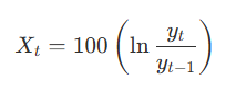
This time-series data is used to calculate a daily standard deviation, which is annualized by multiplying by the square root of the trading days in a year (e.g., 250, 260, or 365 days). This annualization assumes that serial correlation in daily rate moves is negligible.

To translate an annualized yield volatility percentage into basis points (bps), analysts scale it by the prevailing interest rate level. For example, if a bond trades at a yield of 3.00% and features a historical yield volatility of 20%, its annual standard deviation is 60 basis points (20%×3.00%).

Implied Yield Volatility

Rather than relying on backward-looking data, implied volatility is extracted from the market prices of interest-rate options, such as swaptions, caps, and floors. Implied volatility represents the forward-looking volatility parameter that, when input into an option pricing model (such as the Black-Scholes-Merton or Black model), equates the model’s theoretical value to the observed market price.

The Volatility Skew and Smile: If the standard BSM model were perfectly accurate, implied volatility would remain constant across all strike prices. In reality, when plotted against the strike price, implied volatility displays a U-shaped volatility smile or asymmetric smirk (often called a “sneer” in cap markets), indicating that implied volatility is systematically higher for out-of-the-money and in-the-money options than at-the-money options.
The Volatility Surface and Cube: To map this multi-dimensional pricing, dealers construct three-dimensional volatility surfaces (plotting volatility against expiration and strike price) and volatility cubes (which add the underlying swap tenor as a third dimension) to price swaptions and caps accurately.

3. Forecasting Yield Volatility

Because yield volatility varies dynamically over time, researchers rely on advanced statistical models to forecast future volatility:

Stylized Facts: Empirical rate markets exhibit volatility clustering (or persistence)—where large rate changes are clustered together and quiet periods follow quiet periods. Over time, these highly volatile periods exhibit mean reversion, eventually decaying back toward a long-term historical normal level.
Exponentially Weighted Moving Averages (EWMA): Unlike simple moving averages that weigh all past observations equally, EWMA (popularized by RiskMetrics) assigns exponentially declining weights to older observations to prioritize recent market movements in the forecast.
ARCH and GARCH Models: Developed by Robert Engle and Tim Bollerslev, Autoregressive Conditional Heteroscedasticity (ARCH) and Generalized ARCH (GARCH) models mathematically capture volatility clustering and conditional variance by modeling today’s variance (σ ²_t) as a function of both past squared residual deviations from the mean and past estimated variances.

4. Volatility in Option-Embedded Bonds and Term Structure Models

Option-Embedded Bonds

For complex securities whose cash flows are contingent on future interest rates (such as callable corporate bonds, putable corporate bonds, or mortgage-backed securities), volatility is a direct driver of value.

The Option Component: A higher interest-rate volatility assumption systematically increases the value of embedded options. For callable bonds (which represent a long straight bond minus an issuer call option), higher volatility increases the call option’s value, reducing the callable bond’s overall price. For putable bonds (which represent a long straight bond plus an investor put option), higher volatility increases the put option’s value, driving up the putable bond’s price. Similarly, the price of a cap embedded in a capped floating-rate note increases with volatility, reducing the floater’s value.
Option-Adjusted Spread (OAS): Because of this optionality, the OAS of a callable or putable bond is highly sensitive to the volatility assumed in the binomial interest rate tree. Increasing the volatility input increases the value of an embedded call, which reduces the calculated OAS for a callable bond.

Convexity, Volatility, and the Yield Curve

Long Convexity is Long Volatility: Portfolio managers who hold highly convex portfolios (such as barbells) over bullet portfolios are contractually “long volatility”. Because positive convexity adds a positive pricing increment under rate shocks, a highly convex barbell portfolio will outperform a bullet portfolio of matching duration if yields move up or down by a large enough margin. However, highly convex portfolios trade at a lower cash-flow yield (the “cost of convexity”). If rates stay the same or move very little, the low-convexity bullet portfolio will outperform due to its higher yield. Thus, the choice to buy convexity is a direct bet on future interest rate volatility.
Convexity and the Term Structure: In a multi-period setting, interest rate volatility interacts with bond convexity to directly alter the shape of the yield curve. In a risk-neutral world with flat rate expectations, the presence of interest rate volatility causes the term structure of forward rates to slope downward over longer maturities due to the compounding price benefit of positive convexity.

Term Structure Models and Volatility Curves

Vasicek Model: Captures mean reversion but assumes a constant local volatility of the short rate (σ). This specification results in a strictly downward-sloping volatility curve (σe^−kt), which fails to capture the low volatility of very short-term rates typically pegged by central banks.
Gauss+ Model: Overcomes this by modeling three factors (short-rate r, medium-term factor m, and long-term factor l ) but utilizing only two stochastic sources of risk (dW¹ and dW² ). By omitting a volatility term in the short-rate equation, the Gauss+ model is able to match empirical, hump-shaped term structures of volatility where short-term volatility remains low before rising at intermediate maturities.
Shifted-SABR Model: In modern trading of options and swaptions under negative rate regimes, practitioners utilize the shifted-SABR model. By using a shift parameter (b) alongside stochastic volatility parameters (α, β, ρ), this model accommodates negative interest rates while accurately fitting the observed volatility skew and smile across different option strikes and tenors.

Historical Return Volatility

In fixed-income analysis, volatility is fundamentally split into two main branches: yield volatility (interest rate fluctuations, which serve as crucial inputs to term structure and option valuation models) and return volatility (the actual dispersion of realized prices or portfolio returns over an evaluation period). While yield volatility measures the uncertainty of changing interest rates themselves, historical return volatility is designed to evaluate the risk profile of a portfolio manager’s realized performance by analyzing the variation and distribution of past returns.

According to the sources, fully capturing and evaluating historical return volatility requires analyzing the return distribution across three distinct pillars: dispersion (variation), skewness (asymmetry), and kurtosis (tail heaviness).

1. Measures of Dispersion (Variation)

Dispersion measures quantify how “spread out” a portfolio’s historical returns are. The sources outline several statistical methods used to capture this:

Range and Interquartile Range (IQR): The range is the simplest measure of dispersion (the difference between the highest and lowest historical returns), but it is highly sensitive to extreme outliers. The interquartile range (IQR) addresses this by calculating the difference between the 25th and 75th percentiles, thereby ignoring the most extreme 25% on both ends. However, because the IQR only utilizes a fraction of the data, it fails to capture the full variation of the returns.
Mean Absolute Deviation (MAD): This measures the average absolute deviation of all realized returns from a designated reference return (such as the mean).
Variance and Standard Deviation: These represent the most common measures of dispersion in finance. Standard deviation is the positive square root of variance, returning the risk metric back to the original units of return.
The Symmetrical Drawback (Variance/MAD): Both standard deviation and MAD treat returns above and below the mean symmetrically as “risk”. In reality, investors only view downside deviations as unfavorable; treating outperformance above the mean as a penalty is a significant limitation of these metrics. Furthermore, standard deviation assumes a normal distribution, whereas empirical bond returns are consistently non-normally distributed.
Downside Risk Metrics (Semi-variance and LPM): To isolate “bad” volatility, analysts utilize semi-variance (and semi-standard deviation), which completely ignores squared deviations of returns that fall above the mean. To avoid treating the mean as the baseline, the Lower Partial Moment (LPM) is used. The LPM allows investors to choose a customized target “minimum acceptable” reference return, and utilizes a parameter order () to dictate how heavily extreme losses are penalized in risk models.

2. Skewness (Asymmetry)

Skewness measures the asymmetry of the historical return distribution.

Unlike variance, skewness can take on both positive and negative values because the direction of the deviation is important.
If a portfolio’s mean return is located in the left half of the return distribution, it is left-skewed. This is highly critical in fixed income, as a left-skewed distribution indicates that there are more extreme negative returns on the left side than extreme positive returns on the right.

3. Kurtosis (Tail Heaviness)

Kurtosis measures indicate whether the tails of a return distribution are heavy or “fat” compared to a normal distribution (which has a kurtosis of 3).

Excess kurtosis is used to show kurtosis relative to this normal benchmark.
A positive excess kurtosis indicates heavy tails, meaning there is a much higher probability of extreme events (such as sudden default shocks or market dislocations) than a standard normal distribution would predict. In return distributions, the left tail represents direct downside risk.

4. Benchmark Volatility: Backward-Looking Tracking Error

In bond portfolio management, performance is typically measured relative to a benchmark index rather than in isolation. Under this relative context, historical return volatility is quantified using backward-looking tracking error (or ex-post tracking error). This is calculated as the standard deviation of the portfolio’s active returns (portfolio actual return minus benchmark actual return).

5. Integration into Risk-Adjusted Return Ratios

These historical return volatility measures serve as the direct risk denominators for classical reward-to-risk ratios:

The Sharpe Ratio uses standard deviation as its risk measure, but is heavily criticized for penalizing upside outperformance and failing to account for the non-normal skewness and fat tails of bond returns.
The Sortino Ratio replaces standard deviation with “bad” volatility, using the standard deviation of realized returns that fall strictly below a client-specified Minimum Acceptable Return (MAR).
The Information Ratio uses backward-looking tracking error in the denominator to measure active return (alpha) achieved per unit of active risk assumed.

Contrast with Yield Volatility

The broader “context of volatility” also includes yield volatility, which is conceptually different from return volatility. Yield volatility is the standard deviation of the percentage change in yields between two dates.

A portfolio manager must monitor both return and yield volatility. For example, lower-rated corporate bonds (high-yield) generally have a lower duration (meaning lower analytical sensitivity to interest rate changes), which might make them seem less risky. However, because high-yield bonds have far greater yield volatility—as credit spreads fluctuate wildly even when Treasury rates are stable—they can expose investors to massive price and return volatility despite their lower duration.

Implied Yield Volatility

In fixed-income mathematics and portfolio management, volatility is evaluated across two distinct branches: historical return volatility (the realized dispersion of past asset or portfolio returns) and yield volatility (the fluctuation of interest rates themselves). Within yield volatility, analysts distinguish between historical yield volatility—which measures backward-looking standard deviations of daily log-rate changes—and implied yield volatility, which is a forward-looking metric derived directly from the market prices of option-related derivatives.

The provided sources detail the mechanisms, structural behavior, and critical role of implied yield volatility within the broader context of risk measurement and option-adjusted pricing.

1. The Mechanism of Implied Volatility and “Calibration”

Implied yield volatility is a by-product of option pricing models (such as the Black-Scholes-Merton or Black models). The pricing of an interest-rate option is driven by several known inputs: the current price of the underlying bond, the strike price, the time to expiration, the risk-free rate, and the coupon rate. The expected volatility over the option’s life is the only unknown factor.

To estimate this unknown volatility, practitioners assume the current market price of the option is fair and perform implicit estimation (or calibration). By inputting the observed option price along with the known variables, they solve the option pricing model in reverse to back out the implied yield volatility. This is the expected volatility parameter that equates the model’s theoretical price to the actual market price of the option.

Because trading in option markets fundamentally centers on buying and selling expected interest-rate volatility, implied volatility serves as the primary currency for comparing relative value across different option contracts.

2. Analytical Discrepancies and Model Limitations

While implied volatility provides a real-time gauge of forward-looking market expectations, the sources highlight several structural issues with relying solely on it:

Model Dependence: Implied volatility assumes that the underlying option pricing model (and its assumptions) is entirely correct. If the model is flawed, the backed-out implied volatility is mathematically distorted.
The Constant-Volatility Paradox: Most classic option pricing models assume that yield volatility is constant over the life of the option. In reality, as a bond approaches maturity, its price volatility naturally decays toward zero.
Non-Uniform Volatilities: Theoretically, if a model is perfect, implied volatilities for different options written on the exact same underlying bond should be identical. In practice, implied volatilities vary significantly depending on the option type (call or put), the time to expiration, and the strike price.

3. The Volatility Skew, Smile, and “Sneer”

When implied volatility is plotted against the strike price for options with the same expiration, it is rarely flat. This variation is known as the volatility skew.

The Volatility Smile: In equity and currency markets, this plot typically forms a symmetrical, U-shaped curve where implied volatility is higher for in-the-money (ITM) and out-of-the-money (OTM) options than for at-the-money (ATM) options.
The Volatility “Sneer” (or Smirk): For interest-rate options (such as caps and floors), empirical research reveals that the U-shape is asymmetric. ITM caps exhibit a significantly stronger skew than OTM caps, creating a pattern that researchers refer to as a “sneer”.
Surfaces and Cubes: To navigate these pricing discrepancies, dealers construct three-dimensional implied volatility surfaces, which plot implied volatility against both the strike price and the time to expiration. In the swaptions market, this is expanded into a multi-dimensional volatility cube by incorporating the underlying swap tenor as a third dimension.

4. Volatility in Negative Interest Rate Regimes: Shifted-SABR

Under normal circumstances, lognormal interest rate trees are used because they restrict rates from turning negative (since interest-rate changes become smaller as rates approach zero). However, when negative interest rates emerged in Europe and Japan, traditional lognormal models broke down.

To accommodate this, practitioners transitioned to the shifted-SABR model. By adding a deterministic shift parameter (), the model allows the short-term rate to become negative while keeping the local volatility positive. The model’s parameters—including (which matches the ATM swaption volatility), (which controls the fatness of the tails and the volatility smile), and (which manages the correlation between rate changes and volatility changes)—are calibrated to accurately map the observed volatility skew across the interest rate market.

5. The Role of Volatility in Fixed-Income Portfolio Risk

Implied volatility is not merely an input for options; it is a critical driver of the pricing and risk metrics of broader fixed-income portfolios:

Option-Adjusted Spread (OAS) Sensitivity: For bonds with embedded options (like callable or putable corporate debt), the OAS is highly volatility-dependent. For a callable bond, a higher expected volatility increases the value of the issuer’s embedded call option. Since the option value is subtracted from the straight bond value, higher volatility reduces the callable bond’s price, which in turn compresses its calculated OAS. For a putable bond, a higher volatility assumption increases the value of the investor’s put option, raising the bond’s price and increasing its OAS.
Convexity as a Volatility Play: Portfolio managers who actively manage duration must decide whether to pay a premium for positive convexity (e.g., choosing a highly convex barbell portfolio over a bullet portfolio). A highly convex portfolio outperforms in environments with large interest rate movements, but it suffers a lower yield under stable rates. Thus, the decision to hold positive convexity is a direct, structural bet on future interest rate volatility.

Tracking Error (Backward-looking)

In the context of fixed-income return and volatility analysis, backward-looking tracking error (also referred to as ex-post tracking error or tracking risk) is a fundamental statistical measure used to quantify a portfolio’s return volatility relative to a benchmark index.

While traditional measures of dispersion (such as standard deviation or variance) evaluate volatility by measuring deviations around a portfolio’s own historical mean, tracking error specifically measures the volatility of the net active position (the portfolio’s performance relative to its designated benchmark).

The sources detail how backward-looking tracking error is defined, used to adjust returns for risk, and decomposed to manage portfolio volatility:

1. Definition and Mathematical Foundation

The Active Return Standard Deviation: Mathematically, tracking error is defined as the standard deviation of the portfolio’s active return, where active return is the actual portfolio return minus the benchmark index’s return.
The Baseline of Zero: A portfolio that perfectly replicates its benchmark (such as a pure index fund) will have active returns of zero every period, resulting in a tracking error of zero. The closer a portfolio’s tracking error is to zero, the more closely its risk profile matches the risk profile of its benchmark.
Economic Interpretation: Because tracking error is a standard deviation, it can be used to establish a confidence interval for active returns. For example, a tracking error of 30 basis points (bps) indicates that, assuming a normal distribution, the portfolio’s return will fall within bps of the benchmark’s return in approximately two-thirds (68.3%) of the periods.

2. The Risk-Adjusted Reward Context: The Information Ratio

In performance evaluation, backward-looking tracking error serves as the risk denominator for the Information Ratio, a key reward-to-risk metric.

The Information Ratio is calculated as:

where the numerator (alpha) is the average active return over a specified period.

By dividing active outperformance by the historical volatility of that outperformance, the ratio measures how much excess return a manager generated per unit of active risk assumed. In practice, an Information Ratio in the range of 0.40 to 0.60 is historically viewed as “good” performance, while reaching 1.00 over long evaluation horizons is highly rare.

3. Decomposing Relative Volatility: Systematic vs. Idiosyncratic Risk

When managing a portfolio against an index, focusing on standalone portfolio volatility can be highly misleading. A portfolio can appear perfectly stable in isolation but still carry massive tracking error if its holdings mismatch the benchmark’s primary risk factors.

To address this, risk-management frameworks decompose tracking error into two orthogonal (independent) components:

Systematic Tracking Error: The active volatility resulting from mismatches in systematic risk factors, such as yield-curve duration, sector weightings, or credit spread duration (DTS) relative to the benchmark.
Idiosyncratic Tracking Error: The residual, non-systematic volatility specific to individual bond issues or names in the portfolio.
Because systematic and idiosyncratic risks are statistically independent, total tracking error is calculated as the square root of the sum of their squares:

$\text{Portfolio Tracking Error} = \sqrt{(\text{Systematic TE})^2 + (\text{Idiosyncratic TE})^2}$

This decomposition reveals that portfolios with very few holdings (which are less diversified and thus expose the manager to significant name-specific risk) will have their total tracking error dominated by idiosyncratic volatility. In contrast, large benchmark sectors like Treasury securities contribute significantly to systematic tracking error due to active yield-curve duration mismatches, but they contribute almost no idiosyncratic tracking error because their individual returns are highly explained by systematic factors.

4. Backward-Looking vs. Forward-Looking Volatility

The sources emphasize a distinct boundary between the two forms of tracking error:

Backward-Looking (Ex-Post): This is calculated using historical realized active returns to evaluate past performance, calculate the Information Ratio, and conduct attribution analysis.
Forward-Looking (Ex-Ante or Predictive): This is calculated using multifactor risk models and covariance matrices to forecast the future tracking error of a current portfolio structure. Portfolio managers utilize quadratic programming to minimize this predicted tracking error under strict risk budgets and investment constraints.

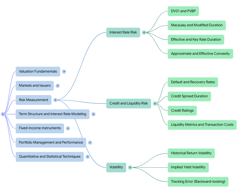
— Linden Lake

This series:
→　Topic Review (1 of 7): Fixed Income – Valuation Fundamentals
→　Topic Review (2 of 7): Fixed Income – Markets and Issuers
→　Topic Review (3 of 7): Fixed Income – Risk Measurement
→　Topic Review (4 of 7): Fixed Income – Term Structure and Interest Rate Modeling
→　Topic Review (5 of 7): Fixed Income – Fixed-Income Instruments
→　Topic Review (6 of 7): Fixed Income – Portfolio Management and Performance
→　Topic Review (7 of 7): Fixed Income – Quantitative and Statistical Techniques

References:
Reference 1, Reference 2, Reference 3

Topic Review (3 of 7): Fixed Income – Risk Measurement

Interest Rate Risk

DV01 and PVBP

Macaulay and Modified Duration

Effective and Key Rate Duration

Approximate and Effective Convexity

Credit and Liquidity Risk

Default and Recovery Rates

Credit Spread Duration

Credit Ratings

Liquidity Metrics and Transaction Costs

Volatility

Historical Return Volatility

Implied Yield Volatility

Tracking Error (Backward-looking)

Leave a Reply Cancel reply