Topic Review (1 of 7): Fixed Income – Valuation Fundamentals

In the study of fixed-income securities, valuation serves as the bridge between raw contractual terms, financial mathematics, and market-driven pricing. Across the analytical frameworks of Frank J. Fabozzi, Bruce Tuckman, and the CFA Institute, valuation is examined through three levels of complexity: traditional single-rate discounting, the arbitrage-free spot/forward curve framework, and advanced probabilistic models for complex securities.

1. The Foundational Rule: Time Value of Money (TVM)

The most basic axiom of financial analysis is that money has a time value because of the opportunity to invest capital and earn interest over time. Consequently, the price of any financial instrument is equal to the present value of its expected future cash flows.

Performing a rigorous valuation of a bond requires two essential steps:

Estimating the size and exact timing of the expected future cash flows.
Determining the appropriate required yield (or discount rate) that reflects the risk of the cash flows relative to comparable investments in the market.

2. Traditional Bond Pricing and the “Pull to Par”

For a traditional, option-free bond, the cash flows are legally fixed and consist of a periodic stream of interest payments (representing an ordinary annuity) and a lump-sum principal repayment at maturity.

The conventional valuation method discounts these cash flows using a single, uniform market discount rate, typically called the yield to maturity (YTM). This relationship establishes fundamental price-yield rules:

Par Bonds: When the coupon rate equals the required yield, the bond trades exactly at its par (face) value.
Discount Bonds: When the coupon rate is below the required yield, the bond trades at a discount to par.
Premium Bonds: When the coupon rate is above the required yield, the bond trades at a premium to par.

If the required yield remains unchanged over the bond’s life, the price of the bond will change solely due to the passage of time. This is illustrated by the constant-yield price trajectory, which depicts the “pull to par” effect: as a bond moves closer to maturity, the premium or discount is gradually amortized away, and the bond’s carrying value converges precisely to par at maturity.

3. The Arbitrage-Free Framework: “A Bond is a Package of Zeros”

While YTM is a convenient shorthand for quoting prices, modern fixed-income mathematics rejects the single-discount-rate approach as theoretically incomplete because it implicitly assumes a flat yield curve. In reality, “a bond is not a bond”—it is a package of zero-coupon instruments maturing at different dates.

Under the arbitrage-free valuation framework, each individual cash flow is treated as an independent zero-coupon security and must be discounted using a rate unique to its specific delivery date. This unique rate is called the spot rate.

This method is deemed “arbitrage-free” due to the Law of One Price, which states that identical assets must sell for the same price. In highly liquid markets, sovereign bonds can be separated into their constituent interest and principal payments via stripping (creating C-STRIPS and P-STRIPS) or combined through reconstitution. If a bond’s market price deviates from its spot-discounted “no-arbitrage value,” a market participant can purchase the cheaper asset, strip or reconstitute it, sell the parts, and lock in a riskless, self-financing arbitrage profit.

Spot rates are mathematically intertwined with implied forward rates—the break-even interest rates agreed upon today for loans to be executed in future periods. When the spot yield curve is upward-sloping, the forward curve lies above the spot curve; when the spot curve is downward-sloping, the forward curve lies below it. Discounting cash flows using either spot rates or their corresponding implied forward rates yields mathematically identical arbitrage-free bond prices.

4. Yield Measures vs. Realized Horizon Returns

A critical theme across the sources is that a bond’s yield to maturity is a “promised yield” that rarely coincides with the actual realized return earned by an investor. The YTM is only fully realized if two highly restrictive conditions are met:

The bond is held until its final maturity date.
All intermediate coupon payments can be reinvested at an interest rate exactly equal to the YTM.

In highly volatile interest rate environments, the assumption of reinvesting at the YTM is deeply unrealistic. For example, if rates drop significantly, coupons are reinvested at much lower rates, causing the investor’s realized return to fall below the promised YTM.

To evaluate performance over shorter horizons, analysts calculate the total return (or horizon yield). This measure incorporates explicit expectations for the coupon reinvestment rate and estimates the bond’s future sale price based on its projected position on the constant-yield trajectory. This analysis highlights the fundamental tension in fixed-income investing between two offsetting risks:

Coupon Reinvestment Risk: The risk that future coupon payments must be reinvested at lower rates.
Market Price Risk: The risk that interest rates will rise, depressing the bond’s sale price before maturity.

5. Fixed-Income Mathematics: Price Volatility, Duration, and Convexity

To manage the trade-off between price risk and reinvestment risk, analysts rely on mathematical derivatives of the price-yield relationship:

Price Value of a Basis Point (DV01 or PV01): The absolute dollar change in a bond’s price resulting from a one-basis-point (0.01%) shift in the yield.
Macaulay Duration: The weighted average of the time to receive all cash flows, where the weights are the present value of each cash flow as a proportion of the total bond price. For zero-coupon bonds, Macaulay duration is exactly equal to maturity; for coupon bonds, it is always shorter.
Modified Duration: A direct linear estimate of the percentage change in a bond’s price for a given change in yield.

Because the underlying price-yield curve of an option-free bond is convex (curved) rather than linear, modified duration is only accurate for very small interest rate shifts. For larger interest rate shifts, modified duration understates price increases when rates fall and overstates price decreases when rates rise. To correct for this, mathematicians calculate convexity—the second derivative of the price-yield function. Combining duration (the first-order approximation) with convexity (the second-order approximation) provides an exceptionally accurate estimate of a bond’s price change.

These risk metrics are the engine of classical portfolio immunization. When an investor’s investment horizon matches a bond’s Macaulay duration, the duration gap is zero: any loss stemming from market price risk is exactly offset by gains from coupon reinvestment risk (and vice versa), locking in the target return.

6. Advanced Valuation: Lattice Models and Embedded Options

Traditional valuation methods collapse entirely when applied to bonds with embedded options (such as callable or putable provisions) or variable coupons (capped and floored floaters). Because the cash flows of these complex securities are interest rate dependent, changes in interest rates alter the probability of option exercise, thereby changing the timing and size of the cash flows themselves.

To value these instruments, modern fixed-income mathematics utilizes arbitrage-free lattice models (such as the binomial interest rate tree):

Calibrating the Tree: A multi-period tree of potential future short-term interest rates is constructed based on an assumed interest rate volatility. The tree is calibrated to be “arbitrage-free” by ensuring that when option-free benchmark bonds are priced on the tree, their model-derived values perfectly match their actual market prices.
Backward Induction: Valuation begins at maturity (where the cash flows are known with certainty) and works backward from right to left through the nodes.
Option Rules: At each node, the model checks whether option exercise is optimal. For example, the issuer will call a bond if the present value of its future cash flows exceeds the strike call price.

This framework allows a bond with embedded options to be mathematically decomposed into its basic parts:

Price of Callable Bond = Price of Straight Bond − Price of Issuer Call Option

Price of Putable Bond = Price of Straight Bond + Price of Investor Put Option

Similarly, when default risk is present, analysts utilize the Option-Adjusted Spread (OAS). The OAS is the constant spread that must be added uniformly to all of the forward rates on the binomial tree to make the model-calculated price of the risky callable/putable bond equal to its observed market price.

Finally, because the cash flows of option-embedded bonds vary as interest rates are shocked, traditional yield-based duration and convexity cannot be used. Instead, analysts must calculate effective duration and effective convexity. These metrics require revaluing the option-embedded bond on newly generated, shocked interest rate trees while keeping the OAS constant, capturing the true, dynamic interest rate sensitivity of the security.

Time Value of Money

The concept of the Time Value of Money (TVM) is the absolute foundation of fixed-income analysis. Money has a time value because of the opportunity to invest capital at an interest rate and earn a return over time. In the broader context of valuation, this fundamental principle dictates that the price of any financial instrument is equal to the present value of its expected future cash flows. Valuation is therefore the practical application of TVM, requiring an analyst to estimate the timing and size of future cash flows and discount them to the present.

1. Fundamental Properties of Discounting (Present Value)

Discounting is the core TVM mechanism used to convert future cash flows into today’s dollars. The sources outline several essential mathematical properties of present value (PV):

The Interest Rate (Discount Rate) Effect: For any given future value, the higher the discount rate, the lower its present value. This is because a higher interest rate allows a smaller sum invested today to grow to the same target future amount over time.
The Time Effect: For a given interest rate, the farther into the future a cash flow is received, the lower its present value. More time allows more interest to accumulate, meaning fewer dollars need to be set aside today to realize that future sum.
Continuous Compounding: In specialized pricing models, interest can be compounded continuously. The TVM formulas adjust such that the future value is FV=Pe^(i×N) and the present value is PV=FVe^(−i×N) (where is the base of the natural logarithm, is the interest rate, and is the number of years).

2. Arbitrage-Free Valuation and the Law of One Price

While traditional finance often relies on a single discount rate to value a bond, modern fixed-income mathematics utilizes discount factors and spot rates to achieve an arbitrage-free valuation.

A discount factor d(t) represents the exact present value of one unit of currency to be received at a specified future date . Reflecting the time value of money, discount factors must decrease as the term increases (assuming positive interest rates).
Under the Law of One Price, identical cash flows must sell for the same price in frictionless markets.
Therefore, modern valuation views a coupon bond not as a single instrument, but as a package of zero-coupon instruments. Discounting each individual cash flow by its maturity-matched spot rate (the yield on a zero-coupon bond) prevents risk-free arbitrage profits through stripping or reconstitution.
Discounting in this manner is mathematically identical to arbitrage pricing (using a replicating portfolio), meaning that discounting cash flows is simply shorthand for arbitrage pricing.

3. Yield Measures and the TVM Reinvestment Assumption

The yield to maturity (YTM) is the single, uniform interest rate that equates the present value of a bond’s promised cash flows to its market price. However, YTM is merely a “promised yield” that is rarely equal to the actual realized return earned by an investor. YTM relies on two restrictive TVM assumptions:

The bond is held until its final maturity date.
All intermediate coupon payments are reinvested at an interest rate exactly equal to the calculated YTM.

Because interest rates fluctuate, the assumption that coupons can be continuously reinvested at the YTM is deeply unrealistic. To bypass these restrictions, analysts calculate the realized horizon return (or total return). This TVM measure incorporates explicit, customized projections for the coupon reinvestment rate over the holding period and estimates the bond’s future sale price based on its projected position on the constant-yield price trajectory.

4. Advanced TVM: Volatility, Convexity, and Lattice Models

When interest rates are volatile, traditional static TVM calculations break down for securities with embedded options (such as callable or putable bonds) because their cash flows are interest-rate dependent.

To value these complex instruments, fixed-income mathematics uses arbitrage-free lattice models (binomial interest rate trees) to represent possible future interest rates based on assumed volatility.
Valuation relies on backward induction: starting at maturity (where the terminal payoff of par and the final coupon are certain) and working backward from right to left through the nodes to find the present value today.
At each node, the bond’s value is the present value of the expected cash flows one period forward, discounted using the node’s specific forward rate.
Additionally, interest rate volatility interacts with the convexity of the price-rate curve. By Jensen’s Inequality, the expected price of a bond under volatility is higher than its price at the expected interest rate (E[1/(1+r)]>1/(1+E[r])). This “convexity advantage” directly lowers implied forward rates relative to expected future spot rates.

Future Value

In fixed-income mathematics and the broader framework of the Time Value of Money (TVM), Future Value (FV) represents the amount to which a current investment will grow over a specified future period when allowed to earn a given rate of interest. Money possesses a time value precisely because of the opportunity to invest capital and earn interest.

The sources outline the mathematical principles, compounding variations, and practical applications of Future Value within fixed-income analysis:

1. The Fundamental Single-Payment Formula

For a single current investment (the principal, P) held for N years at an annual interest rate (expressed as a decimal), the future value is calculated as:

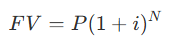
The expression (1+i)^N is known as the future value of $1. This calculation demonstrates that the future value of an investment is composed of three distinct economic components:

The original principal.
The simple interest earned on the principal.
The interest-on-interest (or compound interest) earned by reinvesting intermediate interest payments over the holding period.

For example, an investment of $1,000 at a 7% annual interest rate over 8 years grows to a future value of $1,718.19. Of the $718.19 in total interest, $560 represents simple interest ($70 per year 8 years), while the remaining $158.19 is the interest-on-interest generated by reinvesting those annual cash flows.

2. Adjusting for Compounding Frequency and Fractional Terms

Fractional Periods: The future value formula remains mathematically identical for fractional parts of a year, where is expressed as a decimal (e.g., for an investment spanning 7 years and 3 months).
Compounding Multiple Times per Year: If interest is paid times per year, the future value formula is adjusted by dividing the annual interest rate by and multiplying the number of years by to determine the total number of compounding periods (n=N×m):

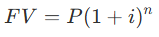
More frequent compounding (e.g., semiannual or quarterly vs. annual) provides a higher future value because it creates more frequent opportunities to reinvest the interest payments.

Continuous Compounding: In specialized models assuming that interest is paid and reinvested at every instant, the future value is computed using the base of the natural logarithm (e):

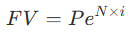
3. Future Value of an Ordinary Annuity

When a series of equal cash flows (A) is paid or received periodically, it is called an annuity. If the first payment occurs one period from now, it is defined as an ordinary annuity. The future value of an ordinary annuity is formulated as:

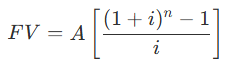
The bracketed expression represents the future value of an ordinary annuity of $1. Bond portfolio managers utilize this formula to calculate the future value of periodic coupon payments and their accumulated reinvestment interest.

4. Future Value in Bond Return Analysis (Total Return)

A bond investor’s total return relies heavily on the future value of intermediate coupon payments.

Interest-on-Interest: By applying the future value of an annuity formula to periodic coupons, analysts calculate the “coupon interest plus interest-on-interest”. This interest-on-interest can represent over 80% of a bond’s potential dollar return for long-term or high-coupon securities.
Total Future Amount: To evaluate a bond’s performance over a specific horizon, analysts calculate the total future amount. If the bond is held to maturity, this future value is the sum of the par value and the accumulated coupon payments plus interest-on-interest. If sold prior to maturity, the total future amount includes the coupons, interest-on-interest, and the estimated future price of the bond at the horizon date.

Present Value

Building on our previous discussions of the Time Value of Money (TVM) and Future Value, we now look at the reverse process: Present Value (PV).

If Future Value tells us how much a sum invested today will grow to over time, Present Value answers the fundamental question of how much money must be invested today to realize a specific, targeted sum in the future. Within fixed-income analysis, this calculation is critical because the fair price of any financial instrument is simply the present value of its expected future cash flows.

The sources systematically explain the mathematical foundations of Present Value, its core properties, its behavior under varying compounding frequencies, and how modern finance uses it to establish an arbitrage-free pricing framework.

1. The Core Present Value Formula and “Discounting”

The process of determining the present value of a future sum is mathematically defined as discounting. Consequently, the present value is often referred to as the discounted value, and the interest rate used to perform this adjustment is known as the discount rate.

To find the present value (PV) of a single future amount (FV) to be received years from today, given an annual interest rate (), the fundamental formula is:

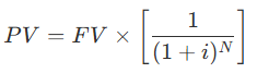
The term in the brackets, 1/{(1+i)^N} , is mathematically defined as the present value of $1. Multiplying this factor by the actual future sum yields the present value of that specific sum.

2. Core Properties of Present Value

The discounted value of any future cash flow is dynamically governed by two fundamental relationships:

The Interest Rate (Discount Rate) Effect (Inverse Relationship): For any given future value at a fixed point in time, the higher the discount rate, the lower the present value. This is because a higher interest rate allows capital to grow at a faster rate; therefore, a smaller sum needs to be invested today to reach the same future target.
The Time Effect (Inverse Relationship): For a given interest rate, the farther into the future a cash flow is received, the lower its present value. When the future payment is delayed, there is more time for interest to accumulate, meaning fewer dollars must be set aside today.

3. Present Value of Multiple Payments and compounding Frequency

Most financial contracts or liabilities do not consist of a single payment, but rather a stream of cash flows.

Summing a Series

To find the present value of a series of future values, an analyst must first calculate the present value of each individual cash flow separately and then sum these present values to arrive at the total present value.

Ordinary Annuities

When the series consists of equal payments received at equal intervals starting one period from today, it is called an ordinary annuity. Rather than discounting each payment individually, the present value of an ordinary annuity of dollars per period for periods can be calculated in a single step:

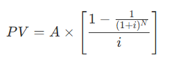
Adjusting for Periodic Compounding

When cash flows are received or paid more than once per year (e.g., times per year, such as semiannually or quarterly), the basic formulas must be adjusted in two ways:

The annual interest rate is divided by the compounding frequency per year (i=annual rate/m).
The number of periods is adjusted by multiplying the number of years by the compounding frequency (n=N×m).

This yields the adjusted formula:

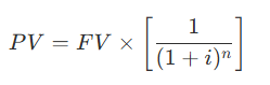
Because cash flows are received more frequently throughout the year, the present value of a bond’s future payments actually increases when payments are made more often (for example, semiannual coupon payments provide a higher present value than annual coupon payments).

Continuous Compounding

In specialized financial models where interest is assumed to compound at every infinite instant, the formula resolves using the natural exponential constant (e):

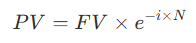
4. Modern TVM: Discount Factors and the Arbitrage-Free Framework

While traditional finance often relies on a single interest rate (like the Yield to Maturity) to discount all cash flows of a multi-period security, modern fixed-income mathematics rejects this single-rate approach as theoretically incomplete. Instead, modern valuation looks at the time value of money through two key concepts:

Discount Factors (d(t))

A discount factor, denoted as d(t) , represents the exact present value of one unit of currency to be received at a specified future date . Discount factors must decline as the term increases (d(0.5)>d(1.0)>d(1.5)). This downward slope is the direct mathematical representation of the time value of money: the longer a payment is delayed, the less it is worth today.

“A Bond is a Package of Zeros”

Under the arbitrage-free valuation framework, a coupon bond is not treated as a single instrument. Rather, it is viewed as a package of zero-coupon instruments maturing at different dates.

To obtain the true, no-arbitrage value of the bond, each individual cash flow must be treated as an independent zero-coupon bond and discounted by its specific, maturity-matched spot rate (the yield on a zero-coupon bond of that exact term):

Replicating Portfolios and the Law of One Price

This method is deemed “arbitrage-free” due to the Law of One Price, which states that identical cash flows must sell for the same price in frictionless markets. If a coupon bond’s market price deviates from the sum of the present values of its cash flows (valued at the spot curve), a market participant can execute stripping or reconstitution to buy the cheaper asset, sell the parts, and lock in a risk-free, self-financing arbitrage profit.

Thus, the mathematical process of discounting future cash flows using spot discount factors is not merely a theoretical exercise—it is the direct mathematical shorthand for arbitrage pricing (replicating the bond’s cash flows with a portfolio of zero-coupon Treasury securities).

Yield (Internal Rate of Return)

In fixed-income mathematics, Yield (specifically the Internal Rate of Return, or IRR) represents the central metric used to summarize, quote, and compare the expected performance of debt instruments. From a Time Value of Money (TVM) perspective, yield is not an arbitrary market quote; rather, it is the mathematically implied discount rate that equates the present value of a security’s expected future cash flows to its current market price.

Across the provided materials, yield is analyzed as a highly intuitive but deeply constrained tool, highlighting its computational mechanics, behavioral relationships, and theoretical limitations.

1. The Mathematical Definition and Computation of Yield (IRR)

The yield (y) on any investment is the uniform interest rate that satisfies the fundamental TVM pricing equation:

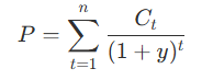
where P is the market price, Ct is the cash flow in period , and is the total number of periods.

Because the cash flows of multi-period securities are distributed across time, solving for the yield (y) generally requires an iterative numerical procedure (trial-and-error search or financial calculator algorithms) to find the exact rate where the total present value of cash flows equals the market price. However, in the special case of an asset that offers only one future cash flow (such as a zero-coupon bond), the yield can be solved directly without iteration using the single-payment formula:

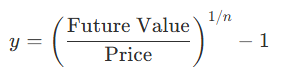
where represents the number of compounding periods.

2. Standardization, Compounding, and Periodicity Conversions

A primary value of yield as an IRR is that it automatically normalizes for both the absolute dollar amount invested and the investment horizon. This allows market participants to compare highly diverse instruments on an intuitive, standardized scale.

However, because bonds pay interest at different intervals (semiannually, quarterly, or annually), yields must be annualized under a defined periodicity (the number of compounding periods per year) to prevent distorted comparisons.

Bond Equivalent Yield (BEY): In the United States, the market convention is to double the semiannual periodic yield to quote the annual rate, known as the bond equivalent yield.
Compounding Conversions: To directly compare bonds with different coupon payment frequencies (such as semiannual vs. quarterly), analysts convert the stated annual percentage rate (APRm) for m periods per year to an equivalent rate (APRn) for n periods per year using the geometric equivalence formula:

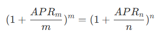
This conversion highlights a core TVM principle: compounding more frequently at a lower annual rate produces the same terminal value as compounding less frequently at a higher annual rate.

3. Yield to Maturity (YTM) and the Restrictive Reinvestment Assumption

For coupon-paying bonds, the most common IRR measure is the yield to maturity (YTM), which represents the promised annualized return if the bond is held to maturity. However, the sources emphasize that YTM is merely a “promised” yield and is rarely equal to the actual realized return earned by an investor.

For the realized holding-period return to perfectly equal the YTM calculated at purchase, three highly restrictive TVM conditions must be met:

Hold to Maturity: The investor must hold the bond until its final maturity date.
No Default: The issuer must make all coupon and principal payments in full and on schedule.
Perfect Reinvestment: All intermediate coupon payments must be continuously reinvested at an interest rate exactly equal to the YTM.

In a dynamic interest rate environment, the reinvestment rate assumption is highly unrealistic. If market interest rates fall, coupons must be reinvested at lower rates, creating reinvestment risk and causing the investor’s actual realized return to fall below the promised YTM. Conversely, if rates rise, the capital loss on a bond sold prior to maturity can easily wipe out the gains from higher coupon reinvestment rates. To manage this trade-off, portfolio managers use total return analysis (or horizon yield), substituting the rigid reinvestment assumptions of YTM with explicit forecasts of future reinvestment rates and ending bond prices.

4. Price-Yield Dynamics and Volatility Properties

Applying a higher or lower yield to the TVM formula yields several fundamental price-yield rules:

The Inverse Relationship: Because a bond’s contractual coupon cash flows are fixed, a bond’s price moves in the opposite direction of its yield.
Premium and Discount Amortization (“Pull to Par”): If the required market yield equals the coupon rate, the bond trades at par. If the required yield rises above the coupon rate, the bond trades at a discount; if the required yield drops below the coupon rate, the bond trades at a premium. Over time, assuming no default, the premium or discount is gradually amortized away, pulling the flat price back to par at maturity.
The Convexity Advantage: The price-yield relationship is not linear, but convex. For an option-free bond, a decrease in yield produces a larger percentage price increase than the percentage price decrease caused by an equal increase in yield.
Coupon and Yield Level Volatility Effects: For a given change in yield, a lower-coupon bond is more price-volatile (has higher duration) than a higher-coupon bond. Furthermore, the lower the prevailing yield level, the greater the price volatility of the bond for a given basis-point shift in rates.

5. Traditional Yield Limitations and the Shift to Arbitrage-Free Frameworks

While convenient, YTM is theoretically incomplete because it assumes a single, flat interest rate applies to all of a bond’s cash flows. In reality, “a bond is a package of zero-coupon instruments” maturing at different dates, and each cash flow should be discounted at the specific spot rate matching its delivery date. Under this modern arbitrage-free framework, a bond’s YTM is simply a complex weighted average of the individual spot rates.

Furthermore, traditional yield-based metrics break down entirely when valuing securities with embedded options (like callable or putable bonds) or variable payments (capped/floored floaters). Because their cash flows are interest-rate dependent, changes in rates alter the likelihood of option exercise, modifying the cash flows themselves. To value these, modern fixed-income mathematics utilizes arbitrage-free lattice models (binomial interest rate trees). These models calibrate possible future short-term forward rates under volatility to ensure the tree matches benchmark par yields. Analysts can then calculate an Option-Adjusted Spread (OAS)—the constant spread added to the tree’s rates to match the model price to the market price—and compute effective duration and convexity to measure true interest rate risk.

Yield (Internal Rate of Return)

Across the provided materials, yield is analyzed as a highly intuitive but deeply constrained tool, highlighting its computational mechanics, behavioral relationships, and theoretical limitations.

1. The Mathematical Definition and Computation of Yield (IRR)

The yield () on any investment is the uniform interest rate that satisfies the fundamental TVM pricing equation: where is the market price, is the cash flow in period , and is the total number of periods.

Because the cash flows of multi-period securities are distributed across time, solving for the yield () generally requires an iterative numerical procedure (trial-and-error search or financial calculator algorithms) to find the exact rate where the total present value of cash flows equals the market price. However, in the special case of an asset that offers only one future cash flow (such as a zero-coupon bond), the yield can be solved directly without iteration using the single-payment formula: where represents the number of compounding periods.

2. Standardization, Compounding, and Periodicity Conversions

Bond Equivalent Yield (BEY): In the United States, the market convention is to double the semiannual periodic yield to quote the annual rate, known as the bond equivalent yield.
Compounding Conversions: To directly compare bonds with different coupon payment frequencies (such as semiannual vs. quarterly), analysts convert the stated annual percentage rate () for periods per year to an equivalent rate () for periods per year using the geometric equivalence formula: This conversion highlights a core TVM principle: compounding more frequently at a lower annual rate produces the same terminal value as compounding less frequently at a higher annual rate.

3. Yield to Maturity (YTM) and the Restrictive Reinvestment Assumption

For the realized holding-period return to perfectly equal the YTM calculated at purchase, three highly restrictive TVM conditions must be met:

Hold to Maturity: The investor must hold the bond until its final maturity date.
No Default: The issuer must make all coupon and principal payments in full and on schedule.
Perfect Reinvestment: All intermediate coupon payments must be continuously reinvested at an interest rate exactly equal to the YTM.

4. Price-Yield Dynamics and Volatility Properties

Applying a higher or lower yield to the TVM formula yields several fundamental price-yield rules:

The Inverse Relationship: Because a bond’s contractual coupon cash flows are fixed, a bond’s price moves in the opposite direction of its yield.
Premium and Discount Amortization (“Pull to Par”): If the required market yield equals the coupon rate, the bond trades at par. If the required yield rises above the coupon rate, the bond trades at a discount; if the required yield drops below the coupon rate, the bond trades at a premium. Over time, assuming no default, the premium or discount is gradually amortized away, pulling the flat price back to par at maturity.
The Convexity Advantage: The price-yield relationship is not linear, but convex. For an option-free bond, a decrease in yield produces a larger percentage price increase than the percentage price decrease caused by an equal increase in yield.
Coupon and Yield Level Volatility Effects: For a given change in yield, a lower-coupon bond is more price-volatile (has higher duration) than a higher-coupon bond. Furthermore, the lower the prevailing yield level, the greater the price volatility of the bond for a given basis-point shift in rates.

5. Traditional Yield Limitations and the Shift to Arbitrage-Free Frameworks

Continuous Compounding

1. Conceptualizing Continuous Compounding

In the broader context of the Time Value of Money (TVM), compounding typically occurs over discrete, defined intervals such as semiannually, quarterly, monthly, or daily. However, continuous compounding represents the extreme mathematical limit of this process, where the number of compounding periods per year approaches infinity. Under this framework, interest is conceptualized as being paid and reinvested at every infinite instant.

While actual bond markets generally trade using periodic semiannual or annual conventions, continuous compounding is widely used in specific practical and theoretical settings:

It is utilized in money markets.
It is frequently employed by financial firms because rates and discount factors often have to be calculated at irregular, non-standard calendar intervals.
It is used almost exclusively by researchers and academic models for mathematical convenience, as it simplifies calculus-based financial derivations.

2. Mathematical Mechanics: Future Value and Present Value

Because interest is compounding continuously, calculations do not use standard periodic compounding exponents. Instead, they rely on the natural exponential constant (the base of the natural logarithm, approximately 2.71828…).

Future Value (FV)

To calculate the future value of an original principal (P) invested for years at an annual interest rate (N) under continuous compounding, the formula is:

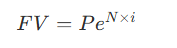
For example, if an investor places $10,000 in an account earning 8% compounded continuously for 1 year, the future value grows to $10,832.87:

Present Value (PV)

To solve for the present value of a target future sum (FV) to be received N years in the future, the formula is worked in reverse (discounted):

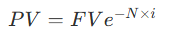
For example, if a manager expects to receive $1,000 in 5 years and requires a 5% return compounded continuously, the present value needed today is $778.80:

3. Continuous Compounding in Advanced Fixed-Income Modeling

Beyond simple single-payment calculations, continuous compounding serves as the mathematical engine for modern term structure modeling, arbitrage pricing, and options valuation:

Discount Factors and Spot Rates: In continuous-time models, the spot rate and the discount factor (the present value of $1 received at time ) are linked directly through a continuous exponential function:

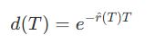
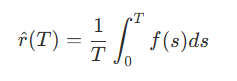
The Spot-Forward Relationship: Rather than using geometric averages of discrete periods, a continuously compounded spot rate over years is represented as the continuous average of the instantaneous forward rates up to that maturity: This continuous representation of forward rates is vital for pricing advanced derivatives, such as interest-rate swaps and caps, and is heavily utilized in proprietary term structure models like the Vasicek and Gauss+ models to describe how the entire yield curve dynamically evolves over time.

Bond Pricing

In the study of fixed-income securities, bond pricing is the primary practical application of the core valuation axiom: the fair price of any financial instrument is equal to the present value of its expected future cash flows. Across the provided materials, this concept is explored through two primary frameworks: traditional single-rate discounting (Yield to Maturity) and modern arbitrage-free discounting (using spot rates), both of which are governed by the mathematical laws of the Time Value of Money (TVM).

1. Traditional Option-Free Bond Pricing Mechanics

Pricing a traditional, option-free bond under the conventional framework is a straightforward discounted cash flow exercise. It requires two key steps:

Estimating Cash Flows: For a standard fixed-rate bond, cash flows consist of a periodic stream of coupon interest payments (which represent an ordinary annuity) and the par value (principal) returned in a lump sum at the maturity date.
Determining the Discount Rate: The cash flows are discounted using a single required interest rate, known as the required yield or yield to maturity (YTM), which reflects the yield demanded by the market for bonds of comparable credit quality and maturity.

The mathematical price of a bond (p) on a coupon date is expressed as:

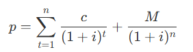
where c is the periodic coupon, M is the maturity value, i is the periodic required yield, and n is the number of periods.

2. Fundamental Price-Yield Relationships

The mathematical structure of the bond pricing formula dictates several immutable rules governing how bond prices behave relative to interest rates:

The Inverse Relationship: Because the promised cash flows (c and M) are contractually fixed, the price of a bond always moves in the opposite direction of its required yield. As the market discount rate increases, the present value of those cash flows decreases, causing the price to fall.
Premium, Discount, and Par Pricing: A bond’s price relative to its par value depends on how its coupon rate compares to the market’s required discount rate:
- Par Bonds: When the coupon rate is exactly equal to the required yield, the bond sells for its par value.
- Discount Bonds: When the coupon rate is less than the required yield, the bond sells at a discount below par. The amount of this discount represents the present value of the coupon “deficiency” relative to what the market demands.
- Premium Bonds: When the coupon rate is higher than the required yield, investors bid the price up to a premium above par. The premium represents the present value of the “excess” coupon cash flows.
The Convexity Effect: The price-yield relationship is not a straight line, but is convex (bowed). For any option-free bond, a given decrease in yield results in a larger percentage price increase than the percentage price decrease caused by an equal increase in yield.
The “Pull to Par” Trajectory: If the required yield remains unchanged over the bond’s life, the price of a premium or discount bond will change solely due to the passage of time. This constant-yield price trajectory pulls the carrying value of a discount bond upward, and amortizes a premium bond downward, until both converge precisely to par on the maturity date.

3. Real-World Conventions: Pricing Between Coupon Dates

In actual debt markets, bonds are rarely traded exactly on coupon payment dates. When a transaction settles between coupon dates, the buyer must compensate the seller for the fraction of the coupon period that the seller held the bond. This introduces the distinction between “clean” and “dirty” prices:

Full (or Dirty) Price: This is the actual cash amount the buyer pays the seller at settlement. It is the true present value of the bond’s remaining cash flows, where the next coupon payment is discounted over a fractional period (1−t/T).
Accrued Interest: The proportional share of the upcoming coupon payment earned by the seller, calculated using standard market day-count conventions (such as actual/actual for Treasuries or 30/360 for corporate bonds). Crucially, accrued interest is calculated linearly and ignores the time value of money.
Flat (or Clean) Price: This is the quoted price that appears on trading screens. It is defined as:

Flat Price = Full Price − Accrued Interest

Dealers quote the clean/flat price to prevent misleading investors; if dealers quoted the full price, the price would appear to rise daily simply because of interest accrual, before dropping precipitously immediately after a coupon payment.

4. Zero-Coupon Bond Valuation

Zero-coupon bonds (like Treasury STRIPS) represent a special, simplified case of bond pricing because they pay no periodic interest. The investor’s return is entirely represented by the difference between the deeply discounted purchase price and the par value received at maturity.

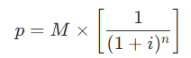
Because there are no intermediate cash flows, the pricing formula collapses to a single present value calculation: p=M×[(1+i)n1] This structural simplicity means zero-coupon bonds have no reinvestment risk, and their price volatility (duration) always scales directly with maturity.

5. The Arbitrage-Free Framework: Spot Rates and Bootstrapping

While YTM is an indispensable trading convention, modern financial theory notes that applying a single discount rate to a multi-period bond is theoretically flawed because the yield curve is rarely flat. Instead, “a bond is not a bond”—it is a package of zero-coupon instruments maturing at different dates.

Under the arbitrage-free valuation framework, each coupon payment and principal repayment is treated as an independent zero-coupon cash flow and is discounted by its own unique maturity-matched spot rate (or “zero rate”):

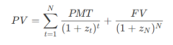
where z_t is the spot rate for period t.

This pricing is strictly bound by the Law of One Price, which dictates that identical cash flows must sell for the same price in frictionless markets. If the market price of a coupon bond deviates from its spot-discounted “no-arbitrage value,” a market participant can purchase the cheaper asset, use stripping or reconstitution to separate or bundle the cash flows, and lock in a risk-free, self-financing arbitrage profit.

Because true zero-coupon government bonds are not always issued across all maturities, analysts derive the theoretical spot curve from observed coupon bond prices using a forward substitution process known as bootstrapping. This ensures that the interest rates used in the pricing model are calibrated to perfectly replicate the observed market prices of benchmark securities, making the entire valuation framework fundamentally arbitrage-free.

Option-Free Pricing

In the study of fixed-income securities, option-free pricing (often referred to as pricing a “straight” or conventional “plain-vanilla” bond) serves as the foundational benchmark for all bond valuation. By definition, an option-free bond contains no embedded contingency provisions (such as call, put, or conversion features) that would allow the issuer or investor to alter its cash flows. Consequently, its promised cash flows are contractually fixed and certain, consisting of a periodic stream of coupon interest payments (an ordinary annuity) and a lump-sum principal repayment at maturity.

The sources analyze option-free pricing through two key valuation frameworks, explaining how this baseline pricing anchors the valuation of much more complex, option-embedded securities.

1. Traditional Pricing: Yield to Maturity (YTM)

The traditional approach to option-free pricing evaluates the bond by discounting all future cash flows using a single required interest rate, known as the market discount rate or yield to maturity (YTM):

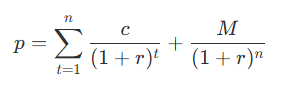
where is the price, is the coupon, is the maturity value, and is the periodic market discount rate. This framework establishes the fundamental rules of bond pricing:

The Inverse Price-Yield Relationship: Because the contractual cash flows of an option-free bond are constant, its price moves in the opposite direction of its yield.
The Convexity Effect: The price-yield relationship of an option-free bond is not a straight line, but is curved, or convex. This positive convexity means that for a given change in yield, the percentage price increase when rates fall is greater than the percentage price decrease when rates rise.
Premium, Discount, and Par Pricing: When the coupon rate equals the required yield, the bond trades at par. If the coupon rate is below the required yield, the bond trades at a discount to compensate the investor for the coupon “deficiency”. If the coupon rate is above the required yield, it trades at a premium.
The “Pull to Par” Effect: Assuming no default and an unchanged required yield over time, the price of a discount or premium bond will move along a constant-yield price trajectory, gradually amortizing the discount or premium until it converges precisely to par value at maturity.

2. Arbitrage-Free Pricing: Spot Rates

While YTM is a universally accepted market shorthand, modern financial theory highlights its limitation: it assumes a flat yield curve by discounting every cash flow at the same rate.

To resolve this, the arbitrage-free valuation framework treats an option-free bond not as a single instrument, but as a package of zero-coupon securities maturing at different dates. Under this framework, each individual cash flow is discounted using a rate unique to its delivery date—the spot rate (or yield to maturity of a risk-free zero-coupon bond):

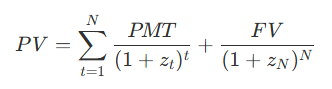
where z_t represents the spot rate for period . This method is termed “arbitrage-free” due to the Law of One Price, which dictates that identical cash flows must sell for the same price in frictionless markets. If a bond’s market price deviates from this spot-discounted “no-arbitrage value,” a market participant can execute stripping (separating coupon and principal payments to trade them as zero-coupon STRIPS) or reconstitution to buy the cheaper asset, sell its constituent parts, and lock in a risk-free, self-financing arbitrage profit.

3. Pricing Option-Free Bonds on a Binomial Lattice

In advanced fixed-income modeling, binomial interest rate trees (lattices) are used to map out potential future interest rate paths. Crucially, the pricing of an option-free bond using a calibrated binomial tree (via backward induction or pathwise valuation) must yield the exact same price as discounting the cash flows directly with spot rates.

Because of this equivalence, option-free pricing serves as the absolute calibration anchor for these mathematical models. To ensure that a binomial lattice is “arbitrage-free” and represents realistic economic conditions, it must first be calibrated such that the interest rates on the tree perfectly price the market’s liquid, option-free benchmark bonds at their observed par or spot values. Only after the tree is calibrated to price option-free bonds correctly can it be trusted to value more complex option-embedded instruments.

4. The Larger Context: Baseline for Option-Embedded Bonds

Option-free bond pricing is the crucial foundation upon which bonds with embedded options (such as callable or putable bonds, capped or floored floaters, and convertibles) are valued. Because these embedded options benefit either the issuer or the investor, they systematically adjust the price relative to the option-free straight bond:

Callable Bonds: A callable bond is viewed as long a straight bond and short a call option sold to the issuer.

Price of Callable Bond=Price of Straight (Option-Free) Bond−Value of Issuer Call Option

Because the option benefits the issuer, a callable bond will always trade at a lower price (and higher yield) than an otherwise identical option-free bond.

Putable Bonds: A putable bond is viewed as long a straight bond and long a put option.

Price of Putable Bond=Price of Straight (Option-Free) Bond+Value of Investor Put Option

Because the option benefits the investor, a putable bond trades at a higher price (and lower yield) than a comparable option-free bond.

Unlike option-free bonds—where cash flows are contractually locked—the cash flows of option-embedded bonds are interest-rate sensitive (declining rates trigger issuer calls; rising rates trigger investor puts). To value these complex structures, analysts use the calibrated binomial lattice. At each node on the tree, the model calculates what the straight option-free cash flows would be, compares them to the option’s strike price, and overrides the straight value if the option is expected to be rationally exercised.

Thus, without the precise mathematical foundation of option-free spot and par rate pricing, calibrating interest rate trees and stripping out the true value of embedded options would be mathematically impossible.

Full vs. Flat Price

In fixed-income markets, when a bond transaction is executed between coupon payment dates, the price paid by the buyer is split into two distinct concepts: the full (or dirty/invoice) price and the flat (or clean/quoted) price.

1. The Core Mechanics

The relationship between these two pricing measures is defined by the following formula:

Full Price=Flat Price+Accrued Interest

The Full Price represents the actual cash amount the buyer pays the seller on the settlement date. It is the mathematically precise present value of the bond’s remaining expected future cash flows. It is referred to as “dirty” because it includes the accrued interest representing the coupon portion the seller has earned by holding the bond for a fraction of the current coupon period.
The Flat Price is the clean quoted price that appears on trading screens and is used to negotiate transactions. It is the full price minus the accrued interest.
Accrued Interest (AI) is the undiscounted, proportional share of the upcoming coupon payment that has accumulated linearly since the last coupon date. It compensates the seller for the days they held the bond during the current period.

2. The Rationale: Why Quoted Prices Are “Flat”

If the buyer always pays the full price at settlement, why does the market convention dictate quoting the flat price? The reason is to avoid misleading investors about the bond’s actual price trend.

Even if market interest rates remain completely constant, the full price of a bond behaves in a cyclical, jagged pattern:

Between coupon dates, the full price rises day by day as the next cash flow draws closer in time and its present value increases.
Immediately after a coupon date, the full price drops precipitously by the exact amount of the coupon payment because that cash flow has just been paid and is no longer part of the bond’s future value.

If dealers quoted the full price, the price would appear to rise continuously before plunging on the coupon date, masking the real impact of interest rate changes. By subtracting the linearly growing accrued interest, the flat price changes only gradually over time. It filters out the noise of coupon accumulation, remaining clean of “coupon-drop” distortions. Thus, the flat price is the carrying value that is actually “pulled to par” along the constant-yield trajectory.

3. Key Analytical and Valuation Subtleties

Beyond daily trading conventions, the full vs. flat distinction introduces critical mathematical nuances in bond valuation:

The Reinvestment & Time Value of Money (TVM) Bias: When calculating the full price, the upcoming coupon payment is discounted back to the settlement date (a discounted value). However, accrued interest is calculated as a simple, linear proportion of the upcoming coupon payment without discounting (an undiscounted value). Because the accrued interest convention ignores TVM, the reported accrued interest is theoretically a little “too high,” and consequently, the flat price is slightly “too low”.
The Impact on Par Bonds and Yield: Because of this undiscounted accrued interest convention, if a bond is priced at par between coupon dates, its yield-to-maturity will actually be slightly less than the coupon rate. The yield only equals the coupon rate for a bond selling at par when the settlement date coincides exactly with a coupon date.
Bonds Trading “Flat”: In certain situations, accrued interest is completely omitted from the transaction. Bonds in default or income bonds trade “flat”—meaning the buyer pays the quoted price without any added accrued interest because future coupon payments are highly uncertain or non-existent.
Global Quoting Differences: While quoting clean (flat) prices is the standard market convention in the United States, some international non-U.S. markets quote the dirty (full) price on trading screens.

Accrued Interest

In fixed-income markets, accrued interest is a vital component of bond pricing that accounts for the fraction of a coupon period that has elapsed since the last coupon payment. Because bonds are routinely traded between scheduled coupon dates, accrued interest ensures that the seller is fairly compensated for the interest earned during their holding period, while the buyer inherits the right to collect the full upcoming coupon payment from the issuer.

1. The Core Definition and Mathematical Formula

Accrued interest is the proportional share of the next coupon payment that has accumulated since the previous coupon date. Mathematically, it is calculated linearly as:

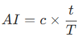
where AI is the accrued interest, c is the periodic coupon payment, t is the number of days from the last coupon payment to the settlement (or value) date, and T is the total number of days in the coupon period.

Interest typically accrues from and including the date of the previous coupon up to but excluding the value/settlement date. However, accrued interest is not computed for all bonds; debt instruments that are currently in default or issued as income bonds trade without accrued interest, which is known as trading flat.

2. Day-Count Conventions and Calculation Variations

To calculate the exact fraction of the coupon period that has elapsed (t/T), markets rely on standardized day-count conventions that vary by security type:

Actual/Actual (In Period): Primarily used for government coupon bonds (such as U.S. Treasury securities). This convention counts the actual number of calendar days between the relevant dates. For instance, if a Treasury bond is settled 138 days into a coupon period that actually spans 184 days, the accrued interest is calculated using a fraction of 138/184.
30/360: Typically used for corporate, municipal, and federal agency securities. This convention assumes that every month has exactly 30 days and the year has 360 days. Under this method, a transaction settled on June 18 when the last coupon was on March 19 would assume exactly 89 days have elapsed (11 days remaining in March, 60 days for April and May, and 18 days in June) out of a standardized 180-day coupon period.

3. Pricing Context: Clean vs. Dirty Prices

In the broader context of bond pricing, accrued interest marks the dividing line between how bonds are quoted and how they are paid for:

The Clean (or Flat) Price: This is the quoted price that appears on trading screens. Quoting clean prices prevents investors from being misled by a bond’s price trend; if dirty prices were quoted, the price would appear to rise daily simply because of interest accrual, before dropping sharply immediately after a coupon payment. Subtracting accrued interest leaves a flat price that changes gradually and is “pulled to par” along the constant-yield trajectory as maturity approaches.
The Dirty (or Full) Price: This is the actual cash amount the buyer pays the seller at settlement. It represents the true present value of the bond’s remaining cash flows.

Thus, the transaction relationship is defined as:

Dirty Price=Clean Price+Accrued Interest

Furthermore, when performing analytical risk calculations like Macaulay duration, the total present value (PVTCF) of the cash flows must be equated to the bond’s full (dirty) price, not the flat price.

4. The Time Value of Money (TVM) Bias and the Par Bond Anomaly

A major mathematical subtlety of accrued interest is its departure from the time value of money.

In bond pricing, the dirty price is calculated by discounting all future cash flows—meaning the upcoming coupon payment is a discounted present value. In contrast, the market convention dictates that accrued interest is calculated linearly and without any discounting. Because the seller receives their share of the coupon cash immediately at settlement rather than waiting until the coupon date, receiving an undiscounted portion means the reported accrued interest is theoretically a little “too high” and the quoted flat price is slightly “too low”.

This undiscounted convention creates a well-known market anomaly: if a bond trades at par between coupon dates, its yield-to-maturity will be slightly less than its coupon rate. The yield only equals the coupon rate for a bond selling at par when the settlement date falls exactly on a coupon payment date, when accrued interest is zero.

5. Dividend Status: Cum-Dividend vs. Ex-Dividend Trading

Finally, the allocation of accrued interest depends on the dividend status of the transaction:

Cum-Dividend (Cum-Coupon): The buyer receives the upcoming coupon, and the buyer must pay the seller accrued interest to compensate them for the days they held the bond.
Ex-Dividend (Ex-Coupon): The seller retains the right to receive the upcoming coupon because the trade occurs during an ex-coupon period. In this case, the seller must compensate the buyer by paying them accrued interest.

While some international markets allow ex-dividend trading, bonds in the United States always trade cum-dividend, meaning the buyer always pays the seller accrued interest.

Matrix Pricing

1. The Structural Need for Matrix Pricing

In the broader context of financial markets, bond pricing is inherently more complex than equity pricing due to the structural differences between the two asset classes. While a typical corporation issues only one class of common stock that trades on a centralized, highly liquid exchange, the same corporation can have multiple debt liabilities outstanding with different maturities, coupon rates, seniorities, and covenants.

Furthermore, unlike equities, the vast majority of bonds are traded in decentralized, over-the-counter (OTC) markets through dealer networks. This fragmentation means that many corporate bond issues do not trade on a daily basis, resulting in “stale” prices. When an analyst or portfolio manager needs to determine the price or yield of a bond that is illiquid, rarely traded, or not yet issued in the primary market, they must rely on matrix pricing.

2. Definition and Core Methodology

Matrix pricing is an appraisal or estimation process used to determine the market discount rate (required yield-to-maturity) and the flat (clean) price of an illiquid or unissued bond. This estimation is constructed using the observed market prices and yields of more actively and frequently traded comparable bonds.

To execute matrix pricing, an analyst follows a structured, multi-step process:

Identify Comparable Bonds: Locate actively traded bonds of similar credit quality (same credit rating), similar coupon rates, and comparable maturities to the target bond.
Determine Yields-to-Maturity: Calculate the yields-to-maturity (implied market discount rates) of these comparable bonds based on their active market prices.
Perform Linear Interpolation: Since comparable bonds rarely have the exact maturity of the target bond, the analyst uses linear interpolation across maturities to estimate the required yield (market discount rate) for the target bond’s exact maturity.
Discount Expected Cash Flows: Once the estimated yield-to-maturity is established, it serves as the market discount rate to discount the target bond’s scheduled cash flows (periodic coupon payments and the final principal repayment at maturity), thereby determining its estimated arbitrage-free price.

For example, if an analyst needs to value an illiquid 4-year corporate bond, they might identify a comparable 3-year bond and a 5-year bond of the same credit quality. By calculating the yields-to-maturity of the 3-year and 5-year bonds, they can linearly interpolate to find the estimated 4-year yield, and then use that rate to price the 4-year bond’s cash flows.

3. Key Applications in Fixed-Income Analysis

Matrix pricing plays three critical roles across different areas of fixed-income portfolio management and primary markets:

A. Valuing Illiquid Portfolio Holdings and Stale Securities

Many institutional portfolios and mutual funds hold corporate debt that trades infrequently. Because fund managers must mark their portfolios to market regularly, they use matrix pricing to establish an appraised “fair value” for these illiquid assets in the absence of recent transaction data.

B. Pricing Bond Market Indices

Broad fixed-income indices (such as the Scotia Capital Universe Bond Index) consist of thousands of individual securities, a large portion of which do not trade on any given day. Rather than using outdated, historical transaction prices, index providers utilize matrix pricing as an appraisal approach to estimate the current market value of these constituents based on their specific characteristics (e.g., sector, coupon, maturity, and credit rating), ensuring the index’s total return and Net Asset Value (NAV) are calculated accurately.

C. Underwriting New Bond Issues

In the primary market, when a corporate issuer is preparing to launch a new bond, investment banks must price the issue appropriately relative to investor demand. Underwriters use matrix pricing to estimate the required yield spread (or spread over the benchmark) that the market will demand. The benchmark is typically the yield-to-maturity on an on-the-run government bond of comparable maturity. The resulting spread represents the risk premium investors require to compensate them for the target bond’s credit risk, liquidity risk, and tax status relative to the “risk-free” benchmark.

4. Limitations and the Broader Valuation Context

In the broader context of fixed-income mathematics, matrix pricing is valued as an elegant and highly practical tool, but it has recognized limitations:

Linearity Assumption: Matrix pricing relies on linear interpolation, which assumes that the yield spread or the credit spread curve moves in a straight line between the selected maturity points. In reality, the term structure of credit spreads is dynamic and can exhibit steepness, twists, and curvature changes that a simple linear matrix model fails to capture.
Equal Seniority Assumption: To price a bond accurately using comparable securities, the bonds must have equal priority in the event of default (i.e., they must be pari passu). If the comparable bonds have different seniorities, covenants, or recovery rates, the matrix pricing estimate will be distorted.
Liquidity Premiums: Traditional structural and reduced-form pricing models assume frictionless markets. In practice, matrix pricing can struggle to separate an issuer’s true credit risk spread from the unique liquidity premium associated with the specific benchmark or comparable bonds used in the grid.

Arbitrage-Free Framework

The arbitrage-free framework represents the mathematical cornerstone of modern fixed-income valuation. In the larger context of valuation fundamentals—which dictate that the value of any financial asset is the present value of its expected future cash flows—the arbitrage-free framework establishes a self-consistent method for pricing both traditional and option-embedded securities by ensuring that market prices adjust to eliminate any opportunities for riskless profit.

1. The Core Economic Axioms

Underpinning this framework are three fundamental economic principles:

The Law of One Price: This rule states that identical assets, or assets that are perfect substitutes, must sell for the exact same price in frictionless markets.
Value Additivity: This principle dictates that “the value of the whole must equal the sum of the values of the parts”. If a portfolio is priced cheaper than its individual underlying components, an investor can buy the portfolio, sell the parts, and lock in a risk-free profit.
Dominance: A risk-free asset that pays off a positive amount in the future must have a positive price today. If a risk-free asset is priced cheaper than another asset with a lower payoff, investors will buy the dominating asset and sell the dominated one until prices align.

Ultimately, the absence of arbitrage opportunities implies that if an investor invests zero net capital today and takes zero risk, their expected return must be zero.

2. Traditional Bond Pricing: “A Bond is a Package of Zeros”

Traditional valuation approaches often discount all of a bond’s cash flows using a single, uniform market discount rate, such as the yield to maturity (YTM), which implicitly and unrealistically assumes a flat yield curve.

Modern arbitrage-free theory rejects this, stating instead that “a bond is not a bond”—it is a package of zero-coupon instruments maturing at different points in time. Consequently, each individual cash flow must be treated as a distinct zero-coupon bond and discounted by its own unique, maturity-matched spot rate. These spot rates are derived from observed par curves of highly liquid benchmark securities (like Treasury issues) through a forward substitution process known as bootstrapping.

If a coupon bond’s market price deviates from this spot-discounted “no-arbitrage value,” a dealer can buy the cheaper asset, use stripping or reconstitution to separate or bundle the coupon and principal components, and lock in a risk-free, self-financing arbitrage profit.

3. Replicating Portfolios and Arbitrage Pricing

The mathematical process of discounting future cash flows is actually a shorthand representation of the much more robust arbitrage pricing (or replication) methodology.

To value a derivative or non-benchmark security, an analyst constructs a replicating portfolio of liquid benchmark assets (such as spot-market zero-coupon bonds) that perfectly mimics the target security’s cash flows under all possible future scenarios. By the Law of One Price, the fair price of the security must equal the current market cost of this replicating portfolio.

If the security is mispriced (trading “rich” or “cheap”), arbitrageurs will immediately execute a self-financing trade—buying the undervalued asset and shorting the overvalued replicating portfolio—which generates risk-free profits today with completely netted future obligations. These collective market forces are what continuously enforce the Law of One Price and push securities toward their arbitrage-free values.

4. The Power of Risk-Neutral Pricing

A major mathematical breakthrough of the arbitrage-free framework is that the price of a derivative does not depend directly on the real-world probabilities of interest rate movements or investors’ risk preferences. Replicating portfolios are identical regardless of whether a rate increase has a 20% or an 80% probability of occurring.

To simplify valuation, the framework utilizes risk-neutral pricing. Instead of building complex physical replicating portfolios for every security, analysts adjust the real-world interest rate probabilities to “risk-neutral probabilities”. These risk-neutral probabilities are calibrated so that the expected discounted values of the underlying assets perfectly match their current cash-market prices. The derivative can then be valued simply as the expected discounted payoff under these risk-neutral probabilities, yielding the exact same price as the replication method.

5. Dynamic Term Structure Models: Lattices and Calibration

While spot rates work perfectly for option-free bonds, they fail to value bonds with embedded options (such as callable or putable bonds, capped or floored floaters, and mortgage products). Because the options’ cash flows are interest-rate dependent, changes in interest rates alter the probability of option exercise and change the timing and size of the cash flows themselves.

To value these, the arbitrage-free framework relies on binomial interest rate trees (lattices), which represent potential future short-rate paths over regular time steps under assumed interest-rate volatility.

Model Calibration: To be “arbitrage-free,” the interest rate tree must be calibrated to ensure that the model-derived prices of liquid, option-free benchmark bonds perfectly match their observed market prices. This calibration process (adding “drift” adjustments) ensures the tree is anchored to real-world economic conditions.
Valuation: Once calibrated, analysts use backward induction—working from right to left through the nodes starting at maturity—to calculate the present value at each node, overlaying rational decision rules to check whether option exercise is optimal. Alternatively, they can use pathwise valuation to discount cash flows along every possible rate path and average the results.
Option-Adjusted Spread (OAS): If a risky option-embedded bond’s market price differs from the model’s calculated price, analysts compute the OAS—the constant spread added to all forward rates on the tree to force the model price to equal the market price.

6. Monte Carlo Simulations for Path-Dependent Cash Flows

For highly complex fixed-income structures like mortgage-backed securities (MBS), cash flows are path-dependent; for example, a homeowner’s decision to prepay a mortgage depends on the historical path interest rates have traveled, not just the current rate.

Because standard binomial trees have no “memory” of past rate paths, the arbitrage-free framework utilizes Monte Carlo methods. This method randomly simulates thousands of interest rate paths. To render the simulation arbitrage-free, a constant drift adjustment is added to all simulated interest rates to force the average present value of the benchmark bonds across all paths to equal their actual market values.

Spot Rates

In the arbitrage-free framework, a spot rate is defined as the annualized yield to maturity on a default-risk-free zero-coupon bond (often called a “zero”) that makes a single payment of principal at maturity. The sequence of these yields across different maturities forms the spot curve (or zero-coupon yield curve), representing the most fundamental structure of interest rates in a given currency.

Modern financial theory and the arbitrage-free valuation framework analyze spot rates through several core dimensions:

1. The “Package of Zeros” Principle

Traditional valuation approaches discount all of a bond’s future cash flows using a single, uniform market discount rate, namely the yield to maturity (YTM). Modern arbitrage-free theory rejects this single-discount-rate approach because it implicitly assumes a flat yield curve. Instead, it establishes that “a bond is not a bond”—it is a package of individual zero-coupon instruments maturing at different dates.

To value a bond in an arbitrage-free manner, each of its individual cash flows must be treated as a distinct zero-coupon security and discounted by the specific spot rate unique to its payment date. Discounting early coupons by a bond’s uniform YTM rather than maturity-matched spot rates introduces pricing errors; for example, with an upward-sloping yield curve, discounting early coupons by the YTM applies too much discounting, understating their true present value.

2. Arbitrage and the Law of One Price

The valuation of a bond as a portfolio of individual cash flows discounted by the spot curve determines its “no-arbitrage value”. Under the Law of One Price, identical assets (or packages of cash flows) must sell for the same price in frictionless markets.

If a coupon bond’s market price deviates from its spot-discounted value, a market participant can generate a riskless, self-financing profit using two primary mechanisms:

Stripping: Separating a coupon bond into its constituent interest payments (creating C-STRIPS or TINTS) and principal payments (creating P-STRIPS), which then trade as independent zero-coupon securities.
Reconstitution: Recombining outstanding zero-coupon STRIPS in the market to recreate the original coupon-paying bond.

If a bond trades in the market for less than its no-arbitrage value, an arbitrageur will purchase the undervalued coupon bond, strip it into individual zero-coupon components, sell those parts at the spot-implied prices, and lock in an immediate, risk-free profit today with zero net future obligations. The collective actions of these arbitrageurs force market prices back into alignment, enforcing the Law of One Price.

3. Deriving Spot Rates through Bootstrapping

Because sovereign entities do not routinely issue zero-coupon bonds across all maturities, the theoretical spot curve must be extracted from the observed prices of actively traded, coupon-paying benchmark bonds. This sequential, forward-substitution process is called bootstrapping.

The mathematical process begins with the shortest maturity:

Year 1: The one-year spot rate (S1) is set equal to the one-year par rate because a one-year bond has only a single terminal cash flow and acts as a pure discount instrument.
Year 2: For a two-year par bond, the two-year spot rate (S2) is solved recursively by equating the bond’s par price of 100 to the present value of its Year 1 coupon (discounted at the known ) and its Year 2 principal plus coupon (discounted at the unknown S2):

Subsequent Years: This substitution is performed sequentially for longer-dated benchmark par bonds to solve for each successive spot rate (S3,S4 , etc.).

To avoid tax biases and liquidity distortions, bootstrapping typically utilizes on-the-run Treasury securities (the most recently auctioned issues), which trade closest to par and possess the highest liquidity.

4. Spot Rates vs. Forward Rates

Spot rates are mathematically tied to implied forward rates—the interest rates agreed upon today for loans to be executed at a specified future date. Specifically, a spot rate is the geometric mean of the current short-term spot rate and the successive implied one-period forward rates leading to that maturity.

Because spot rates and forward rates are mathematically locked, they represent the same underlying time value of money. Consequently, valuing a bond’s cash flows by discounting them with spot rates is mathematically equivalent to discounting them sequentially period-by-period using the corresponding implied forward rates.

5. Calibrating Lattices for Option-Embedded Bonds

While spot curves are sufficient for option-free bonds, they cannot easily value bonds with embedded options (such as callable or putable bonds) because their cash flows are interest-rate dependent. To value these complex structures, modern fixed-income mathematics utilizes calibrated binomial interest rate trees (lattices).

To ensure the valuation is arbitrage-free, the interest rate lattice must be calibrated so that the short-term rates on the tree perfectly price the market’s liquid, option-free benchmark bonds at their observed par or spot values. This calibration constraint is satisfied recursively at each time step by forcing the expected discounted value of the benchmark cash flows under risk-neutral probabilities to equal the spot-rate price of the bond. Once the interest rate tree is calibrated to match the spot curve, it can be reliably used to value option-embedded bonds via backward induction.

Forward Rates

1. Economic Definition and the Forward Rate Model

A forward rate is the interest rate agreed upon today for a loan or bond transaction to be initiated at a designated future date (T∗) for a specified period or tenor (T). Under the arbitrage-free framework, these rates are mathematically derived from the current spot curve. The mathematical relationship is governed by the forward rate model:

where r(T) represents the spot rate for maturity T , and　 f(T∗ ,T) is the implied forward rate.

Spot and forward curves are mathematically locked; they simply present the same underlying time-value-of-money information in different formats. When the spot yield curve is upward-sloping, the forward curve lies above the spot curve; when the spot curve is downward-sloping, the forward curve lies below it.

2. The Breakeven and Replication Principle (Arbitrage Pricing)

In financial mathematics, an implied forward rate represents a “breakeven” reinvestment rate. It is the rate that makes an investor indifferent between:

Purchasing a single, longer-term zero-coupon bond.
Purchasing a shorter-term zero-coupon bond and subsequently reinvesting the proceeds at the forward rate upon maturity.

This indifference is strictly enforced by the Law of One Price and the principle of value additivity. If the market price of a forward contract deviates from the theoretical forward price ,

a risk-free, self-financing arbitrage opportunity is created.

For example, if a forward bond price is underpriced in the market, an arbitrageur can buy the forward contract and simultaneously short a matching synthetic forward position (constructed by purchasing the bond in the spot market and financing it through a repo agreement to the forward date), locking in an immediate, riskless profit.

3. Expected Returns under the “Realized Forwards” Scenario

In active portfolio management, the forward curve provides a baseline for evaluating price and yield changes over time. If the spot curve evolves exactly as predicted by today’s forward rates, the scenario is known as realized forwards (often associated with the pure expectations hypothesis).

Under the realized forward scenario:

The price of an outstanding forward contract remains completely unchanged as time passes.
A bond simply “rolls down” the yield curve.
Most importantly, the holding-period return of any bond or portfolio over a given period is mathematically equal to the short-term risk-free rate for that period (plus its initial option-adjusted or bond spread, if any).

Any deviation in realized returns from the risk-free rate is therefore attributable to rates and spreads shifting away from what was originally implied by the forward curve.

4. One-Period Forward Rates in Binomial Lattices

To value complex securities with interest-rate-dependent cash flows (such as callable or putable bonds, or capped floaters), modern fixed-income mathematics utilizes arbitrage-free binomial lattices.

A binomial interest rate tree is a multi-period graphical depiction of the possible one-period (e.g., six-month or one-year) forward rates over time, based on an assumed interest rate volatility.
To render the tree “arbitrage-free,” it is calibrated (recursively through backward induction) so that the model-determined prices of liquid, option-free benchmark par bonds perfectly match their observed market prices.
Once calibrated, discounting a bond’s cash flows along the tree (either recursively or via pathwise valuation) yields a price mathematically identical to discounting those cash flows directly at spot rates.

5. Forward Rates as “Hedgeable” Rates

Although forward rates are mathematically precise, empirical studies indicate they do not do a good job of predicting future spot rates. Because of this, sophisticated market participants prefer to interpret forward rates not as consensus forecasts, but as hedgeable rates.

By utilizing spot-market securities and financing transactions (such as repo or interest rate swaps), an investor can synthetically lock in the forward rate today, completely hedging their exposure to future interest rate fluctuations. If a portfolio manager’s personal projection of the future spot rate is lower than the hedgeable forward rate, they will buy the bond (perceiving it as cheap); if their projection is higher, they will sell or short it.

6. The Futures-Forward Rate Discrepancy

Under an arbitrage-free term structure, futures rates and forward rates are not identical due to the daily settlement feature of futures contracts.

A forward contract is settled only at expiration, whereas a futures contract is settled daily via margin payments.
When interest rates fall, a long futures position generates early cash profits when reinvestment rates are low; when interest rates rise, it suffers early losses that must be financed at high rates.
Because this daily settlement timing is unfavorable to the contract holder, buyers demand a yield premium.

Consequently, in a rational arbitrage-free model, the implied futures rate of interest always exceeds the corresponding forward rate. This discrepancy increases with the volatility of interest rates and the contract’s term to expiration.

Pathwise Valuation

Within the arbitrage-free valuation framework, pathwise valuation is a mathematically elegant, alternative approach to the traditional backward induction method used to value fixed-income securities on a binomial interest rate tree.

While backward induction works node-by-node from the maturity date back to today, pathwise valuation looks at the interest rate tree as a map of discrete, complete journeys that interest rates can take over time.

1. The Core Mechanics of Pathwise Valuation

An interest rate path is defined as the specific route a short-term interest rate takes from the current time (Time 0) to the security’s maturity. Pathwise valuation calculates the present value of a bond’s cash flows along each of these individual paths and then averages those present values to determine the bond’s fair value.

This approach is executed in three systematic steps:

Specify a list of all potential interest rate paths through the calibrated binomial tree.
Determine the present value of the bond’s cash flows along each individual path. This is done by discounting each period’s cash flow using the specific sequence of one-period forward rates realized along that path.
Calculate the average present value across all possible paths to find the final arbitrage-free price of the bond.

Path Counting and Pascal’s Triangle

The total number of paths in a binomial tree scales over time and can be mapped out using Pascal’s Triangle. For instance, to value a three-year zero-coupon bond, there are four potential interest rate paths to reach Year 3 (HH, HT, TH, and TT, representing combinations of up-steps “H” and down-steps “L” or “T”). For a three-year coupon-bearing bond, there are eight total paths through the tree, which collapse into four unique interest rate combinations.

2. Mathematical Equivalence and Arbitrage-Free Integrity

A defining principle of the arbitrage-free framework is the Law of One Price, which dictates that identical cash flows must sell for the same price to prevent riskless arbitrage. Because a calibrated binomial tree is constructed to be completely arbitrage-free (meaning it perfectly replicates the market prices of option-free benchmark bonds), pathwise valuation must yield the exact same price as the backward induction methodology.

For example, whether a three-year 5% coupon bond is valued node-by-node via backward induction or by averaging the discounted cash flows across its eight distinct rate paths, both methods resolve to the identical arbitrage-free price (e.g., $102.81).

Because of this exact mathematical equivalence, performing both backward induction and pathwise valuation on the same security serves as a primary integrity and calibration test. If both methods do not yield the identical price, it alerts the analyst that the interest rate tree has not been calibrated correctly or is not arbitrage-free.

3. The Bridge to Monte Carlo Simulation

While pathwise valuation is theoretically robust, its primary limitation in the arbitrage-free framework is computational complexity. As the maturity of a security lengthens or the time step is reduced, the number of potential paths grows exponentially. For a 10-year security with semiannual steps, there are over 500,000 paths; for a 20-year security, there are over 500 billion. Evaluating every single path becomes computationally unwieldy.

To overcome this, market participants rely on the Monte Carlo method. Instead of conducting a complete pathwise valuation of every possible path, the Monte Carlo method randomly selects a large, statistically sufficient sample of paths (e.g., 500 or 1,024 paths) from the underlying probability distribution.

This random sampling allows analysts to approximate the results of a complete pathwise valuation within a very tight tolerance (often “within a tick”). This approximation is especially critical for valuing path-dependent fixed-income securities like mortgage-backed securities (MBS), where prepayments and cash flows depend heavily on the historical path interest rates have traveled rather than just the current rate node.

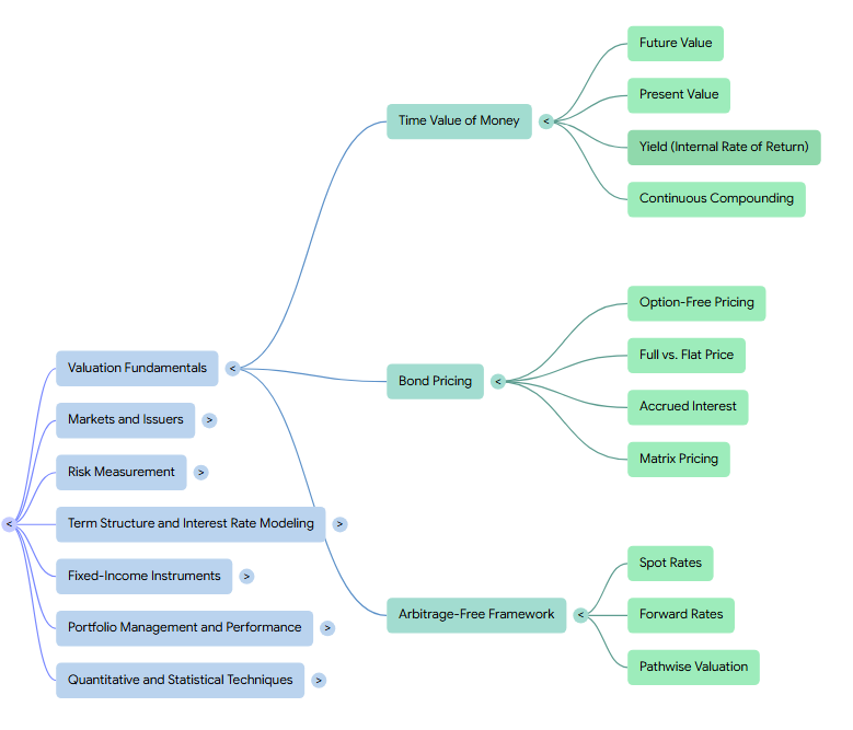
— Linden Lake

This series:
→　Topic Review (1 of 7): Fixed Income – Valuation Fundamentals
→　Topic Review (2 of 7): Fixed Income – Markets and Issuers
→　Topic Review (3 of 7): Fixed Income – Risk Measurement
→　Topic Review (4 of 7): Fixed Income – Term Structure and Interest Rate Modeling
→　Topic Review (5 of 7): Fixed Income – Fixed-Income Instruments
→　Topic Review (6 of 7): Fixed Income – Portfolio Management and Performance
→　Topic Review (7 of 7): Fixed Income – Quantitative and Statistical Techniques

References:
Reference 1, Reference 2, Reference 3

Topic Review (1 of 7): Fixed Income – Valuation Fundamentals

Time Value of Money

Future Value

Present Value

Yield (Internal Rate of Return)

Yield (Internal Rate of Return)

Continuous Compounding

Bond Pricing

Option-Free Pricing

Full vs. Flat Price

Accrued Interest

Matrix Pricing

Arbitrage-Free Framework

Spot Rates

Forward Rates

Pathwise Valuation

Leave a Reply Cancel reply