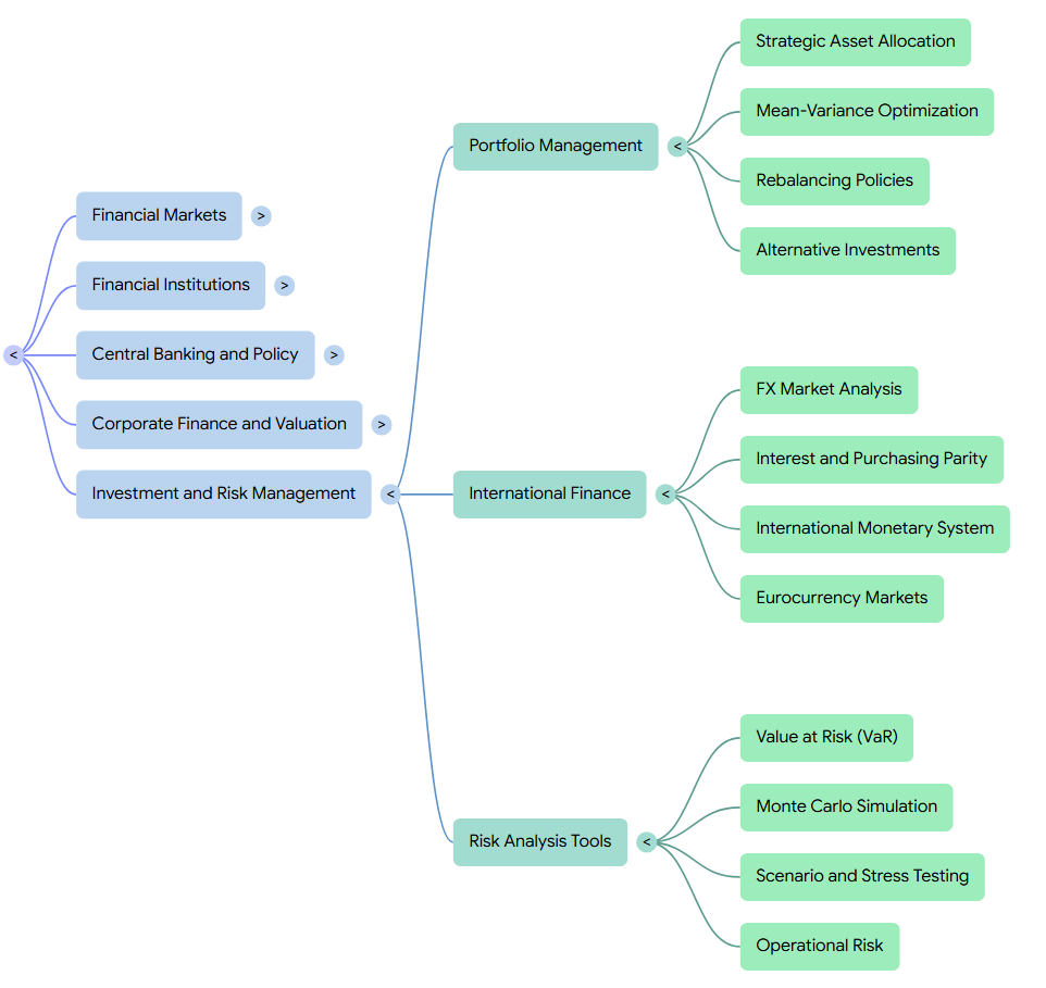
In the integrated landscape of money, banking, and financial markets, investment and risk management are inseparable disciplines. The sources emphasize that financial institutions (FIs) are fundamentally in the “risk management business,” performing the essential function of bearing and managing risk on behalf of customers through risk pooling and specialization.

1. Fundamental Framework of Risk and Return

The core principle of investment is the risk-return trade-off, which holds that in competitive markets, higher expected returns can only be achieved by accepting greater risk.

Systematic vs. Unsystematic Risk: Investors distinguish between systematic (market) risk, which is non-diversifiable and affects all assets, and unsystematic (idiosyncratic) risk, which is unique to a firm or sector and can be eliminated through diversification.
The Capital Asset Pricing Model (CAPM): This model is the primary tool for pricing risk, stating that an investment’s expected return equals the risk-free rate plus a premium based on its beta (β), or its sensitivity to the broader market.
Alpha (α): This represents the “extra” return generated by superior portfolio management beyond what is expected based on the asset’s beta.

2. The Taxonomy of Bank and Market Risks

FIs face a multifaceted inventory of risks that impact their stability and profitability:

Credit Risk: The primary risk in banking, referring to the probability that borrowers will default on promised payments.
Interest Rate Risk (IRR): The uncertainty regarding earnings (Net Interest Income) and economic value (EVE) caused by fluctuations in market interest rates.
Liquidity Risk: The danger of being unable to meet immediate cash demands (funding liquidity) or being forced to sell assets at “fire-sale” prices (asset liquidity).
Market Risk: The risk of loss in the bank’s trading book—assets held for short-term profit—due to changes in prices, FX rates, or interest rates.
Operational Risk: The risk of loss resulting from failed internal processes, people, systems (cybersecurity), or external events like fraud and natural disasters.

3. Investment Portfolio Management Strategies

Firms and individuals manage their investments through structured asset allocation:

Strategic Asset Allocation (SAA): Setting long-term target weights for various asset classes based on risk tolerance and return objectives.
Tactical Asset Allocation (TAA): Making deliberate short-term deviations from the SAA to exploit perceived market inefficiencies or favorable economic conditions.
Passive vs. Active Management: Passive management involves matching a benchmark (e.g., the S&P 500), while active management (fundamental or quantitative) seeks to outperform a benchmark through security selection or market timing.
Fixed Income Maturity Strategies: Banks often use laddered strategies (equal investments across maturities) to reduce income fluctuations or barbell strategies (concentrated short- and long-term holdings) to balance liquidity with high income.

4. Asset-Liability Management (ALM)

ALM is the “beating heart” of a bank, focused on the coordinated management of both sides of the balance sheet.

Gap Management: Banks use GAP analysis to measure the mismatch between interest-sensitive assets and liabilities. A liability-sensitive bank (more rate-sensitive liabilities than assets) risks falling profits if interest rates rise.
Immunization: A strategy of matching the duration of assets and liabilities to shield the bank’s net worth from interest rate shocks.
Derivatives as Hedging Tools: FIs use futures, forwards, options, and swaps to manage risks. For example, a bank can use an Interest Rate Swap (IRS) to convert its fixed-rate loan income into floating-rate receipts to better match its floating-rate deposit costs.

5. Regulatory Framework and Systemic Risk

Because bank failures impose massive negative externalities on the economy, they are subject to heavy regulation.

Basel Accords (I, II, III): These international standards require banks to maintain minimum capital adequacy ratios relative to their risk-weighted assets (RWA).
Systemic Risk: The “ripple effect” where the failure of one large, interconnected institution (a SIFI) threatens the entire financial system.
Macroprudential Supervision: A post-2008 shift where regulators look across the entire financial system—rather than just individual banks—to identify building vulnerabilities.
Stress Testing: The use of doomsday scenarios to ensure banks hold enough capital to survive severe economic contractions, such as the Federal Reserve’s CCAR process.

Portfolio Management

Portfolio management is the integrated process of combining investment assets into a collection that maximizes expected returns for a given level of risk, or minimizes risk for a desired level of return. In the larger context of investment and risk management, it serves as the bridge between individual security analysis and the fulfillment of a client’s long-term financial objectives, such as retirement funding or liability satisfaction.

1. Foundational Principles: Modern Portfolio Theory (MPT)

The core of portfolio management is the principle of diversification, which holds that spreading investments across assets whose returns do not move in lockstep lowers overall risk.

Risk Decomposition: Total portfolio risk is divided into systematic (market) risk, which is inherent in the entire economy and cannot be avoided, and unsystematic (idiosyncratic) risk, which is unique to a specific firm or industry.
The Power of Diversification: While diversification can almost completely eliminate unsystematic risk—typically requiring a portfolio of 25 to 40 diverse stocks—it cannot reduce systematic risk.
The Efficient Frontier: Portfolios that provide the maximum possible return for each level of risk comprise the efficient frontier. Rational investors aim to select a portfolio on this frontier that aligns with their personal risk aversion.

2. Strategic and Tactical Frameworks

Portfolio management is executed through a structured process that begins with the Investment Policy Statement (IPS), a foundational document defining a client’s risk/return objectives and constraints, such as liquidity needs and time horizons.

Strategic Asset Allocation (SAA): This is the long-term “policy portfolio” that sets baseline weights for broad asset classes (e.g., stocks, bonds, real estate). SAA is the primary driver of a portfolio’s long-term risk and return.
Tactical Asset Allocation (TAA): TAA involves making short-term, deliberate deviations from the SAA to exploit perceived market inefficiencies or temporary price dislocations.
Security Selection: This final step involves picking specific individual securities within each asset class to outperform a chosen benchmark.

3. Investment Management Styles

The sources categorize management styles based on their approach to market efficiency and decision-making:

Passive Management (Indexing): Assumes markets are efficient and seeks to replicate the return of a benchmark index at the lowest possible cost. It focuses on capturing beta (market exposure).
Active Management: Assumes markets are inefficient and uses skill to identify mispriced securities to generate alpha (excess return).
Fundamental vs. Quantitative: Fundamental approaches rely on human judgment and in-depth research of individual companies. Quantitative approaches use rules-based models and computer algorithms to systematically search for predictive patterns across vast datasets.

4. Integrated Risk Management Techniques

Risk management in portfolio construction involves active oversight and the use of specialized tools:

Rebalancing: The discipline of periodically adjusting portfolio weights back to the strategic target as market prices fluctuate, which controls intended risk exposures.
Risk Budgeting and Parity: Risk budgeting subdivides the portfolio’s total risk appetite among various sources of return (SAA, TAA, selection). Risk parity goes further, constructing a portfolio where each asset or factor contributes equally to total risk.
Hedging with Derivatives: Managers use futures, options, and swaps to manage exposures without selling underlying assets. For example, equity futures can adjust a portfolio’s beta, and interest rate swaps can hedge the risk of rising rates.

5. Institutional and Liability-Driven Context

For financial institutions, portfolio management is often defined by Asset-Liability Management (ALM), where the goal is to manage the coordinated risk of both sides of the balance sheet.

Liability-Driven Investing (LDI): Common for pension funds and insurers, LDI structures an asset portfolio specifically to fund future liability payments.
Immunization and Matching: Techniques such as duration matching (equating the interest-rate sensitivity of assets and liabilities) and cash flow matching (aligning asset inflows with liability outflows) are used to shield net worth from interest rate shocks.

6. Performance Appraisal

To evaluate the success of portfolio management, several risk-adjusted metrics are employed:

Sharpe Ratio: Measures excess return per unit of total volatility.
Treynor Ratio: Measures excess return per unit of systematic risk (beta).
Information Ratio: Assesses the active manager’s skill by dividing active return by active risk (the tracking error).

Strategic Asset Allocation

Strategic Asset Allocation (SAA), often referred to as the “policy portfolio,” is the process of determining long-term target weights for a set of permissible asset classes based on an investor’s objectives, risk tolerance, and investment constraints. In the broader landscape of portfolio management, SAA is widely considered the most important decision an investor makes, as it serves as the primary determinant of long-run portfolio performance and risk variability.

The Strategic Significance of SAA

SAA serves as the baseline framework for a portfolio, acting as a bridge between an investor’s circumstances and the capital markets.

Driver of Returns: Research indicates that SAA accounts for between 85% and 94% of the differences in total returns for diversified, institutionally managed portfolios.
The “Policy Portfolio” as a Benchmark: The SAA defines the “normal” allocation for the fund and acts as a benchmark against which the value added by active management (security selection and tactical shifts) is measured.
Risk Control: It represents the systematic market risk (beta) an investor is willing to assume to reach their goals, whereas specific return enhancement (alpha) is sought through other means.

The Formulation Process

Developing an SAA is a systematic process that reconciles investor needs with market realities:

Investment Policy Statement (IPS): The process begins by identifying the asset owner’s objectives (return goals and risk tolerance) and constraints (liquidity, time horizon, and tax status).
Capital Market Expectations (CME): Portfolio managers develop long-term forecasts for the risk, return, and correlation prospects of various asset classes.
Optimization and Simulation: Using tools like Mean-Variance Optimization (MVO), managers identify the “Efficient Frontier”—the set of portfolios offering the highest expected return for a given level of risk. The optimal SAA is found at the point where the efficient frontier is tangent to the investor’s highest attainable indifference curve (representing their utility).

Primary Frameworks for Asset Allocation

The sources distinguish three broad approaches to determining an SAA based on how liabilities and goals are treated:

Asset-Only Approach: Focuses exclusively on the asset side of the balance sheet, aiming to maximize the Sharpe ratio for an acceptable level of volatility.
Liability-Relative Approach: Explicitly models liabilities (such as for pension funds or insurers) and focuses on maintaining a healthy surplus or funding ratio. It often uses a “two-bucket” strategy consisting of a hedging portfolio (matching liabilities) and a return-seeking portfolio.
Goals-Based Approach: Disaggregates the portfolio into sub-portfolios, each tailored to a specific goal (e.g., education, retirement, or philanthropy) with its own time horizon and required probability of success.

SAA in Relation to Tactical Asset Allocation (TAA)

While SAA focuses on the long-term, Tactical Asset Allocation (TAA) represents the decision to deliberately and temporarily deviate from SAA targets.

Active Management: TAA is a form of active management at the asset class level, aiming to exploit short-term market inefficiencies or price dislocations.
Risk Profile: Unlike SAA, which reflects equilibrium expectations, TAA moves the investor’s risk away from their targeted long-term profile to capture opportunistic gains.

Portfolio Drift and Rebalancing

The sources emphasize that SAA is not a static decision. Over time, as asset prices fluctuate, the actual allocation will drift from the strategic targets.

Rebalancing Policy: Investors must establish a formal rebalancing discipline to return the portfolio to its SAA weights. This can be calendar-based (e.g., quarterly) or range-based (triggered when an asset class hits a specific corridor limit).
Review Cycle: While implementation vehicles may be reviewed frequently, the SAA itself is typically revisited every few years or upon a significant change in the investor’s goals or global economic fundamentals.

Mean-Variance Optimization

Mean-Variance Optimization (MVO), pioneered by Harry Markowitz in 1952, is the foundational quantitative framework of modern portfolio theory (MPT). In the larger context of portfolio management, MVO provides a mathematical process for constructing “efficient” portfolios that maximize expected return for a given level of risk (volatility) or, conversely, minimize risk for a targeted level of return.

1. The Core Strategic Insight: Diversification

The central tenet of MVO is that an asset should not be evaluated solely on its standalone risk and return, but rather on its contribution to the risk and return of the entire portfolio.

Covariance and Correlation: MVO recognizes that if asset returns are not perfectly correlated, they can be combined to form a portfolio with a lower total variance than the weighted average of the individual assets’ variances.
The “Free Lunch”: By exploiting these correlations, investors can reduce unsystematic (idiosyncratic) risk through diversification, ideally leaving only the systematic (market) risk that cannot be diversified away.

2. The Mechanics of Implementation

To perform MVO, a portfolio manager requires three primary sets of inputs: expected returns, variances (volatilities), and pairwise correlations (or a covariance matrix) for all assets in the opportunity set.

The Utility Function: Optimization is often framed as maximizing an investor’s utility (), which penalizes expected return () based on the portfolio’s variance () and the investor’s level of risk aversion (). A common formula is: .
The Efficient Frontier: By varying the target return or risk, the optimizer traces out the efficient frontier—a curve representing all portfolios that offer the best possible risk-return trade-off. Portfolios falling below this curve are considered “inefficient”.
The Separation Property: In a world with a risk-free asset, James Tobin’s Separation Theorem notes that the task of identifying the optimal risky portfolio (the tangent portfolio) is a technical one, independent of an investor’s personal risk preferences. Investors simply choose their desired risk level by mixing this single tangent portfolio with risk-free borrowing or lending.

3. Tactical Challenges: “Error Maximizers”

While theoretically elegant, MVO is often criticized in practice for its high sensitivity to inputs, earning it the derogatory label of an “error maximizer”.

Input Sensitivity: Small adjustments to expected returns can lead to massive and often “wild” swings in the resulting portfolio weights.
Concentration Risk: Unconstrained MVO frequently produces highly concentrated portfolios that bet heavily on a small subset of assets with the most attractive historical data, which may be the result of estimation error.
Normal Distribution Assumption: MVO assumes returns follow a normal distribution, which fails to account for higher moments like skewness (asymmetry) and kurtosis (fat tails/extreme events), which are prevalent in alternative investments like hedge funds and private equity.

4. Advanced Tactical Mitigants

To overcome these flaws, practitioners employ several advanced modifications:

Constraints: Managers often add non-negativity constraints (prohibiting short sales) or position limits to force the model toward more diversified, realistic results.
Reverse Optimization and Black-Litterman: Reverse optimization starts with market-capitalization weights and “backs out” the implied returns. The Black-Litterman model then allows managers to blend these stable market equilibrium returns with their own unique “views”.
Resampling: Resampled MVO uses Monte Carlo simulation to generate thousands of potential frontiers based on variations in inputs, averaging the results to create a more robust “resampled efficient frontier”.
Shrinkage: This statistical technique “shrinks” extreme historical sample parameters toward a more stable target (like the global mean or a factor model) to reduce the impact of outliers.
Liquidity Penalties: For alternative assets, a liquidity penalty function can be added to the objective function to explicitly penalize assets for being difficult to trade.

Rebalancing Policies

Rebalancing is the discipline of adjusting portfolio weights to more closely align with a client’s Strategic Asset Allocation (SAA). In the larger context of portfolio management, it is a critical component of the monitoring and feedback phase of the investment process. While some market participants may view it as a return-enhancement tool, the sources emphasize that its primary strategic purpose is risk control, ensuring that a portfolio’s risk profile does not drift away from what the investor originally intended.

1. Frameworks for Rebalancing

The sources identify two primary systematic frameworks for implementing a rebalancing policy:

Calendar Rebalancing: This involve adjusting the portfolio to target weights on a periodic basis, such as monthly, quarterly, or annually. It is the simplest approach and involves lower monitoring costs, but the timing is arbitrary and does not react to market volatility between periods.
Percent-Range (Threshold) Rebalancing: This method sets rebalancing corridors or trigger points (e.g., ±5%) around target weights. The portfolio is rebalanced only when an asset class weight breaches these limits. This is considered a more disciplined risk control policy because it is contingent on actual market movements.

2. Strategic Considerations for Corridor Width

When using a percent-range approach, determining the optimal width of the rebalancing corridor involves a trade-off between the costs of transacting and the utility loss from straying from the optimal allocation. Strategic factors influencing corridor width include:

Transaction Costs: Higher costs for an asset class imply wider rebalancing ranges to avoid eroding returns.
Risk Tolerance: More risk-averse investors should have tighter ranges to keep the portfolio closely aligned with their safety requirements.
Correlation: If an asset is highly correlated with the rest of the portfolio, a wider range is permissible because the asset acts as a substitute, and divergences have less impact on overall risk.
Volatility: Higher volatility in the rest of the portfolio points to narrower corridors to prevent large divergences from becoming more likely. For the asset class’s own volatility, there is a trade-off; higher volatility makes divergence more likely (suggesting tighter ranges) but also increases transaction frequency (suggesting wider ranges to control costs).
Tax Considerations: For taxable investors, rebalancing is a discretionary event that triggers capital gains taxes. Consequently, taxable accounts often have wider and asymmetric corridors to minimize tax impact and allow for more aggressive tax-loss harvesting.

3. Tactical Implementation Tools

Portfolio managers have several tactical options for executing rebalancing trades:

Rebalancing back to target vs. range edge: Managers must decide whether to return a weight exactly to the SAA target, only back to the edge of the corridor (to minimize costs), or somewhere in between.
Derivatives Overlays: Institutional investors often use futures or swaps to rebalance “synthetically”. This allows them to adjust the portfolio’s total risk exposure quickly and at a lower cost without disrupting the underlying strategies of active managers.
Exchange-Traded Funds (ETFs): ETFs are useful for rebalancing to target weights in a single trade, providing immediate liquidity and maintaining full investment in the benchmark.

4. Context-Specific Nuances

Fixed-Income Portfolios: Rebalancing is uniquely essential for immunized portfolios. As time passes and interest rates change, the duration and dollar duration (BPV) of assets and liabilities will “drift” at different rates, requiring constant adjustment to maintain the hedge.
Mean-Reversion vs. Momentum: Rebalancing is fundamentally a contrarian approach. It adds the most value in mean-reverting markets—a concept known as “rebalancing yield” or “diversification return”—but can detract from performance in strongly trending markets where it forces the sale of winning assets prematurely.
Goals-Based Investing: In private wealth management, failing to rebalance can lead to a portfolio becoming too conservative over time as higher-priority (low-risk) goal sub-portfolios grow and dominate the total asset mix.

Alternative Investments

In the broader landscape of portfolio management, alternative investments are asset classes that depart from traditional stocks, bonds, and cash in both form and function. While there is no universally accepted definition, the sources generally classify them into four major subclasses: hedge funds, private equity (including venture capital and leveraged buyouts), real assets (such as real estate, commodities, timberland, and farmland), and structured products.

1. The Strategic Roles of Alternatives

Allocations to alternatives have accelerated since the 2008 financial crisis, driven by the belief that they enhance the risk-adjusted return profile of a portfolio. They typically fulfill four functional roles:

Capital Growth: Venture capital and leveraged buyouts (LBOs) act as “return engines,” often providing a premium over public equities to compensate for illiquidity and complexity.
Income Generation: Private credit and certain real estate strategies provide steady cash flow streams.
Risk Diversification: Alternatives often have low correlations with traditional assets, which can shift the efficient frontier up and left, providing a higher Sharpe ratio.
Safety/Inflation Hedging: Real assets like commodities and timber are perceived as hedges against unexpected inflation.

2. Distinctive Characteristics and Challenges

Alternatives differ significantly from traditional assets in several key operational and statistical ways:

Illiquidity: Many alternatives, particularly private equity and direct real estate, require long-term commitments (often 10–14 years) and have restricted redemption windows.
Information Asymmetry and Transparency: Unlike mutual funds, which have strict public reporting requirements, private partnerships provide minimal information about strategy and holdings, often operating as “blind pools”.
Fee Structures: They typically utilize a “2 and 20” model—a 1%–2% management fee plus a 20% incentive fee (carried interest) based on performance beyond a hurdle rate.
Statistical Non-normality: Returns often exhibit serial correlation (price smoothing) due to appraisal-based valuations, which can artificially lower measured volatility and inflate Sharpe ratios. They also frequently display skewness and fat tails (kurtosis), meaning they are more susceptible to rare but extreme “black swan” events.

3. Allocation Models and Frameworks

The sources highlight two dominant paradigms for incorporating alternatives:

The Endowment (Yale) Model: Popularized by David Swensen, this model emphasizes high allocations to illiquid, non-traditional assets (often >50%) and aggressive active management to capture illiquidity premiums.
Risk Factor-Based Approach: This modern lens views assets through their underlying risk exposures (e.g., equity risk, credit spread, liquidity) rather than traditional labels. It helps allocators see that seemingly different assets may share the same primary drivers, thus avoiding a false sense of diversification.

4. Implementation and Access

Investors can access alternatives through various channels depending on their scale and expertise:

Direct Investment: Requires significant in-house resources for due diligence and manager sourcing.
Funds of Funds (FoF): Provides diversified access for smaller or less experienced investors but adds an extra layer of fees.
Liquid Alternatives: Registered vehicles (like alternative mutual funds or ETFs) that attempt to replicate hedge fund strategies with daily liquidity and lower fees, though they are often constrained by regulatory limits on leverage and shorting.

5. Performance Evaluation and Monitoring

Benchmarking alternatives is notoriously difficult due to the lack of high-quality investable indices. Private asset performance is typically measured using the Internal Rate of Return (IRR) or Multiple on Invested Capital (MOIC), though these can be manipulated by the timing of cash flows. For private equity, the Public Market Equivalent (PME) method is used to compare private returns to a hypothetical investment in a public index. Monitoring is labor-intensive and focuses heavily on key person risk and investment strategy drift.

International Finance

International finance is a critical dimension of the globalized and integrated world economy, significantly impacting both investment and risk management strategies. It encompasses the study of the international monetary system, foreign exchange (FX) markets, and the specialized financial management needs of multinational corporations (MNCs) that operate across multiple sovereign jurisdictions.

1. International Investment and Diversification

The primary motivation for international investment is the pursuit of a better risk-return tradeoff than can be achieved through domestic assets alone.

The Power of Diversification: Because national financial markets are influenced by local economic and political factors, they are not perfectly correlated. International diversification allows investors to eliminate unsystematic (country-specific) risk, effectively pushing the efficient frontier “up and to the left”—offering higher returns for the same level of risk.
The Efficient Global Portfolio: Research suggests that a fully diversified international portfolio can be significantly less risky than a purely domestic one. For example, U.S. assets account for less than half of the world portfolio, and forgoing international markets means missing ample opportunities to improve the optimal risky portfolio.
Investment Vehicles: Investors can access international markets through direct purchases, American Depository Receipts (ADRs), internationally diversified mutual funds, Exchange-Traded Funds (ETFs), and closed-end country funds.
Home-Country Bias: Despite the clear benefits, many investors exhibit a strong “home bias,” allocating a disproportionate share of their funds to domestic securities due to perceived lower uncertainty or institutional restrictions.
Emerging Markets: These markets often offer higher growth prospects and lower correlations with developed markets, though they bring unique risks, including political instability, less developed legal protections, and higher volatility.

2. International Risk Management

Managing international financial risk requires identifying and mitigating exposures that do not exist in a purely domestic setting.

A. Foreign Exchange (FX) Risk

FX risk is the uncertainty that exchange rate changes will adversely affect the value of assets, liabilities, or cash flows. It is categorized into three types:

Transaction Exposure: The risk that the realized home-currency value of known, contractually binding foreign currency cash flows (like receivables or payables) will change before they are settled.
Economic (Operating) Exposure: The extent to which a firm’s future operating cash flows—and thus its total market value—are sensitive to unanticipated exchange rate changes that affect its long-term competitive position.
Translation (Accounting) Exposure: The impact of exchange rate changes on a firm’s consolidated financial statements when foreign subsidiary results are converted into the parent’s reporting currency.

B. Country and Sovereign Risk

Country Risk: This encompasses the general political, economic, and social uncertainty within a country that could affect the value of investments or the ability to repatriate profits.
Sovereign Risk: A specific type of credit risk referring to the possibility that a foreign government will default on its debt or interfere with private sector repayments due to currency shortages or political reasons.

3. Hedging Strategies and Parity Conditions

To manage these risks, firms utilize both financial and operational strategies, guided by fundamental parity conditions.

Financial Hedging Tools: Corporations use a variety of derivatives, including FX forwards (to lock in rates), FX futures (standardized exchange-traded contracts), currency options (providing downside protection while retaining upside potential), and currency swaps (to exchange debt-service obligations in different currencies).
Operational Hedging: Long-term strategic adjustments such as multilateral netting of inter-subsidiary payments, leading and lagging (speeding up or slowing down payments based on currency expectations), choosing the invoice currency, and shifting production sites to low-cost or same-currency zones.
International Parity Relationships: These include Interest Rate Parity (IRP) (linking interest rates and forward rates), Purchasing Power Parity (PPP) (linking inflation and exchange rates), and the International Fisher Effect (IFE) (linking interest rates to expected exchange rate changes).

4. Valuation and the Cost of Capital

International finance complicates valuation by requiring decisions on the appropriate discount rate.

Global vs. Local CAPM: If capital markets are fully integrated, a Global CAPM is appropriate, where beta is measured against a global market portfolio. If markets are segmented, a Local CAPM is used.
Weighted Average Cost of Capital (WACC): For foreign projects, the WACC must be adjusted to reflect local tax rates, the effective cost of foreign currency debt, and the specific systematic risk of the project.
Cross-Listing Benefits: Firms in segmented markets can often lower their cost of capital and increase their share price by cross-listing their stock on major global exchanges, thereby making their shares internationally tradable.

FX Market Analysis

In the broader context of international finance, analysis of the Foreign Exchange (FX) market is essential for understanding how capital flows between nations, how international trade is priced, and how multinational corporations (MNCs) manage risk. The FX market is the largest and most liquid financial market in the world, with daily trading volumes exceeding $5 trillion to $6 trillion.

1. Market Structure and Dynamics

The FX market is an over-the-counter (OTC) market, meaning it has no central physical location; instead, it is a worldwide electronic network of banks, dealers, and brokers.

Two-Tier Structure: The market operates on two levels: the wholesale (interbank) market, where large banks trade in huge volumes, and the retail (client) market, where banks service MNCs, money managers, and individuals.
Electronification: Analysis has been transformed by the “electronification” of the market, with over 70% of spot trading now executed electronically. This has led to narrower bid-ask spreads, increased price transparency, and faster adjustment to news.
Vehicle Currencies: The U.S. dollar is the dominant “vehicle currency,” involved in approximately 88% of all global transactions.

2. Frameworks for FX Analysis

Analysts distinguish between exchange rate determination in the long run versus the short run.

Long-Run Analysis: Purchasing Power Parity (PPP)

Long-run analysis focuses on the Law of One Price, which posits that identical goods should cost the same worldwide when expressed in a common currency.

PPP Theory: States that exchange rates adjust to reflect changes in the relative price levels (inflation) of two countries. If a country has higher inflation than its partners, its currency should depreciate.
The Big Mac Index: A popular tool for absolute PPP analysis that compares the price of a standardized product worldwide to see if a currency is over- or undervalued relative to its “correct” PPP level.

Short-Run Analysis: The Asset Market Approach

Short-run analysis treats currencies as financial assets. In this view, exchange rates are determined by the willingness of investors to hold the existing supply of assets denominated in that currency.

Interest Rate Parity (IRP): The central short-run equilibrium condition. It states that the difference in interest rates between two countries must be equal to the difference between the spot and forward exchange rates. If IRP is violated, covered interest arbitrage opportunities arise, which traders quickly exploit to restore equilibrium.
The Role of Expectations: Short-term movements are highly sensitive to “news” and changes in expectations regarding future monetary policy, economic growth, and political stability.

3. Forecasting Methodologies

The sources identify three primary approaches to forecasting exchange rates within an international finance framework:

Efficient Market Approach: Assumes all available information is already reflected in the current spot and forward rates. Therefore, the forward rate is considered the market’s unbiased predictor of the future spot rate.
Fundamental Approach: Uses econometric models based on economic variables like relative money supplies, national output (GDP) growth, and trade balances.
Technical Approach: Ignores economic fundamentals and instead analyzes past price and volume data to identify patterns (e.g., moving average crossovers) that may repeat in the future.

4. Strategic Implementation: The “Trilemma”

In the larger context of international finance, FX market analysis is constrained by the Policy Trilemma (or the “Impossible Trinity”). This principle states that a country cannot simultaneously have:

A fixed exchange rate.
Free capital mobility (unrestricted capital flows).
An independent monetary policy.

Analysts must evaluate which two of these goals a nation has prioritized. For example, the Eurozone allows free capital flow and has an independent central bank (the ECB), but must therefore accept a floating exchange rate. Conversely, countries that fix their exchange rates must often sacrifice monetary independence or impose capital controls.

5. Applications: Exposure and Hedging

For MNCs, FX analysis informs the management of three types of currency exposure:

Transaction Exposure: Risk to contractually binding future cash flows (e.g., payables/receivables).
Translation (Accounting) Exposure: Risk that an unanticipated change in exchange rates will affect the consolidated financial statements of the parent firm.
Operating (Economic) Exposure: The extent to which the total value of the firm (PV of future cash flows) is sensitive to exchange rate changes that impact its global competitiveness.

To manage these, firms use analysis to choose between hedging instruments such as forwards (locking in a rate), futures (standardized exchange-traded contracts), and options (providing downside protection while retaining upside potential).

Interest and Purchasing Parity

In the larger context of international finance, interest rate parity (IRP) and purchasing power parity (PPP) are fundamental equilibrium conditions derived from the law of one price (LOP). These parity relationships serve as the primary frameworks for understanding how exchange rates, interest rates, and inflation rates are inextricably linked across global markets.

1. Purchasing Power Parity (PPP)

PPP is the application of the law of one price to national price levels rather than individual goods. It posits that in the long run, exchange rates adjust to equalize the purchasing power of different currencies.

Absolute PPP: This version states that the exchange rate between two currencies should equal the ratio of the countries’ price levels for a standard basket of goods. A well-known lighthearted illustration of this is the Big Mac Index, which compares the price of an identical burger across nations to judge if a currency is over- or undervalued.
Relative PPP: Because transportation costs and trade barriers prevent absolute price equality, relative PPP focuses on rates of change. It asserts that the percentage change in the exchange rate between two countries over a period will be approximately equal to the difference in their inflation rates.
The Real Exchange Rate: Deviations from PPP result in changes to the real exchange rate, which measures the relative price of domestic goods versus foreign goods. If a country’s currency depreciates by less than its inflation differential, its real exchange rate rises, weakening its international competitiveness.

2. Interest Rate Parity (IRP)

IRP is a no-arbitrage condition that links the spot exchange rate, the forward exchange rate, and the interest rate differential between two countries.

Covered Interest Parity: This holds that the “covered” (hedged) return on a foreign investment must equal the return on a domestic investment of identical risk. If the U.S. interest rate is higher than the U.K. rate, the dollar must sell at a forward discount (meaning the forward rate is higher than the spot rate in terms of dollars per pound) to offset the interest advantage.
Covered Interest Arbitrage (CIA): If IRP is violated, traders can earn risk-free profits by borrowing in the low-interest-rate currency, converting to the high-interest currency, and simultaneously selling the high-interest currency forward to “lock in” the return.
Uncovered Interest Parity (UIP): This asserts that the expected change in the spot exchange rate should equal the nominal interest rate differential. Unlike covered parity, which is enforced by arbitrage, UIP is primarily expectational and often fails to hold in the short run, allowing for strategies like the currency carry trade.

3. The Integrated Parity Framework

International finance uses these parities, along with the Fisher Effect (FE) and the International Fisher Effect (IFE), to create a coherent model of the global economy.

The Fisher Effect: States that nominal interest rates in any country reflect the required real rate of return plus an inflation premium.
The International Fisher Effect (IFE): Combines PPP and the Fisher Effect to suggest that currencies with high nominal interest rates will depreciate because those high rates merely reflect high expected inflation.
Forward Expectations Parity (FEP): Derived when IFE is combined with IRP, this suggests that the forward premium or discount is an unbiased predictor of the future change in the spot exchange rate.

4. Real-World Deviations and Market Dynamics

The sources emphasize that while these parities are elegant in theory, they are rarely exact descriptions of reality due to several factors:

Short-Run Deviations: PPP is a poor predictor of exchange rates over short horizons because goods prices are “sticky” (slow to adjust), whereas nominal exchange rates respond instantly to news. Deviations from PPP typically take three to five years to reduce by half.
Transaction Costs and Capital Controls: IRP may not hold precisely if there are high transaction costs (bid-ask spreads) or if governments impose capital controls that restrict the free flow of funds.
The “Trilemma”: Analysts must recognize that a country cannot simultaneously have a fixed exchange rate, free capital mobility, and an independent monetary policy. Maintaining a fixed rate often requires sacrificing the ability to use interest rates to combat domestic inflation.
Currency Volatility: In a floating regime, exchange rates are often more volatile than the underlying economic fundamentals (like inflation ratios) because they act as financial assets driven by rapidly shifting investor expectations.

International Monetary System

In the broader context of international finance, the international monetary system (IMS) is defined as the institutional framework, agreements, and policies that facilitate international payments, accommodate capital movements, and determine exchange rates among currencies. It provides the essential financial environment in which multinational corporations (MNCs) and international investors operate, directly impacting trade patterns, investment decisions, and global economic stability.

1. Historical Evolution of the IMS

The IMS has evolved through several distinct stages, reflecting shifts in global economic power and political priorities:

Bimetallism (Before 1875): A double standard where both gold and silver were used as international means of payment. This era was often characterized by Gresham’s Law, where the officially overvalued (abundant) metal drove the undervalued (scarce) metal out of circulation.
Classical Gold Standard (1875–1914): Participating nations fixed their currency values in terms of gold and allowed free gold movement. It featured the price-specie-flow mechanism, an automatic adjustment process that corrected balance-of-payments imbalances through gold-driven changes in domestic money supplies and price levels.
Interwar Period (1915–1944): A period of instability marked by hyperinflation in Europe, “beggar-thy-neighbor” competitive devaluations, and the gradual displacement of the British pound by the U.S. dollar as the dominant global currency.
Bretton Woods System (1945–1971): Established at the end of WWII, this was a dollar-based gold-exchange standard. Currencies were pegged to the dollar, which was in turn pegged to gold at $35 per ounce. It collapsed due to U.S. inflation and the Triffin Paradox, which noted that providing global liquidity through U.S. deficits eventually undermined confidence in the dollar.
Flexible Exchange Rate Regime (1973–Present): Following the Jamaica Agreement, exchange rates were allowed to fluctuate based on market forces. Major industrial nations later agreed to the Louvre Accord (1987) to coordinate interventions and achieve greater stability.

2. The “Trilemma” of International Finance

A central concept in designing an IMS is the policy trilemma (or “impossible trinity”), which states that a country cannot simultaneously achieve:

A stable exchange rate.
An independent monetary policy.
Capital market integration (free flow of capital).

Countries must choose two. For example, the Eurozone chooses capital mobility and monetary independence but accepts a volatile exchange rate against external currencies. Conversely, countries with currency boards (like Hong Kong) choose exchange stability and capital mobility but surrender their monetary independence.

3. Current Exchange Rate Regimes

The modern system is a hybrid of several arrangements:

Free Float: Exchange rates are market-determined with minimal intervention (e.g., U.S., Japan, U.K.).
Managed Float (Dirty Float): Central banks intervene to smooth fluctuations without committing to a specific rate (e.g., Brazil, India, Korea).
Fixed Pegs: Currencies are tied to an anchor (usually the dollar or euro). Currency boards and dollarization (adopting a foreign currency as sole legal tender) represent the strongest commitments to fixed rates.

4. Key International Institutions

The IMS relies on several global organizations to maintain order and provide liquidity:

International Monetary Fund (IMF): Originally created to maintain fixed rates, it now acts as a lender of last resort for countries facing currency or balance-of-payments crises. It manages Special Drawing Rights (SDRs), an artificial reserve asset based on a basket of major currencies (USD, EUR, RMB, JPY, GBP).
World Bank: Focuses on long-term project financing and economic development, particularly in poorer nations.
Bank for International Settlements (BIS): Acts as a “central bank for central banks,” fostering cooperation and setting global standards like the Basel Accords on bank capital.

5. European Monetary Integration

A significant development in the IMS is the European Monetary Union (EMU) and the introduction of the euro in 1999. This created an optimum currency area—a region where the benefits of a single currency (lower transaction costs, eliminated exchange risk) are believed to outweigh the costs of losing national monetary policy. However, the European sovereign debt crisis (starting in 2010) highlighted the difficulty of maintaining a single monetary policy across disparate economies with diverging fiscal policies.

6. IMS and Currency Crises

The sources highlight that the IMS’s fragility is often exposed during emerging market crises, such as the Mexican Peso Crisis (1994), the Asian Currency Crisis (1997), and the Argentine Peso Crisis (2002). These events frequently involve speculative attacks where markets force devaluations of overvalued currencies that lack credible policy backing. Managing these risks requires MNCs to utilize hedging tools like forwards, futures, and options within the larger foreign exchange market.

Eurocurrency Markets

In the larger context of international finance, Eurocurrency markets serve as the core of the international money market, providing a massive, parallel banking system that facilitates global capital mobility and the financing of international trade. A Eurocurrency is defined as any freely convertible currency deposited in a bank located outside its country of origin.

1. Fundamental Nature and Misnomers

The sources clarify that the prefix “Euro” is a misnomer; these markets are global in scope. For example, U.S. dollars deposited in London, Singapore, or Hong Kong are all classified as Eurodollars. Similarly, Eurosterling refers to British pounds held outside the United Kingdom, and Euroyen to Japanese yen held outside Japan.

2. Origins and Regulatory Arbitrage

The market originated in the 1950s when Soviet Bloc countries, fearing that their U.S. dollar balances in American banks might be frozen or seized, transferred them to banks in Europe (notably a French bank with the telex address “EURO-BANK”).

The market’s subsequent explosive growth was driven by regulatory arbitrage. By operating offshore, banks (known as Eurobanks) and their customers can bypass several domestic constraints:

Reduced Costs: They are not subject to reserve requirements (such as the Federal Reserve’s Regulation D) or mandatory deposit insurance premiums.
Interest Rate Flexibility: They can escape interest rate ceilings that often prevail in domestic markets.
Efficiency: Transactions are wholesale, typically involving sums of $1 million or more, which allows for narrower borrowing-lending spreads than in domestic systems.

3. Key Instruments and Pricing

The Eurocurrency market functions through two primary activities:

Eurocurrency Deposits: These are typically short-term time deposits or negotiable certificates of deposit (NCDs).
Eurocredits: These are short- to medium-term loans extended to corporations or sovereign governments. They are almost exclusively floating-rate loans.
Reference Rates: Historically, these loans have been priced at a fixed margin over the London Interbank Offered Rate (LIBOR). Other regional rates include EURIBOR (for the euro), SIBOR (Singapore), and TIBOR (Tokyo). Due to recent scandals and structural changes, the market is currently transitioning to new benchmarks like the Secured Overnight Financing Rate (SOFR) in the U.S. and SONIA in the U.K..

4. Eurocurrency vs. Eurobonds

The sources highlight a “fundamental distinction” between these two sectors of the international capital market:

Intermediation: The Eurocurrency market relies on commercial bank intermediation, where banks transform short-term deposits into longer-term claims on borrowers.
Direct Financing: In the Eurobond market, borrowers issue securities directly to final investors.
Maturity and Flexibility: Eurobonds typically have longer maturities, but Eurocurrency loans offer more flexibility, such as the ability to draw down funds in stages or switch currencies on rollover dates via multicurrency clauses.

5. Context within International Finance

Eurocurrency markets play several vital roles in the global financial infrastructure:

Facilitating Trade: They provide the liquid funds necessary for multinational corporations (MNCs) to fund international operations and trade.
Interest Rate Parity (IRP): The market is a primary mechanism for enforcing IRP. Arbitrageurs move funds between domestic and Eurocurrency markets, ensuring that forward exchange premiums or discounts closely reflect interest rate differentials.
Global Liquidity: It acts as a massive pool of offshore funds that can be switched between currencies at the “flick of an electronic blip,” providing firms with more financial options but increasing the complexity of global risk management.
Banking Growth: The market has been a significant stimulus for the expansion of international banking, prompting major U.S. and European banks to open foreign branches to capture offshore deposits.

Risk Analysis Tools

In the integrated world of investment and risk management, risk analysis tools are the quantitative and qualitative mechanisms used to ensure that risks are manageable and that expected returns are commensurate with the level of uncertainty assumed. These tools allow financial institutions and investors to identify, assess, monitor, and control exposures across a broad spectrum, including market, credit, liquidity, and operational risks.

Core Statistical Risk Measures

Statistical tools provide a common language for quantifying the “total risk” of a portfolio by compressing complex variables into single metrics.

Value at Risk (VaR): The most ubiquitous tool, VaR estimates the maximum potential loss over a specific time interval (e.g., one day) at a given confidence level (e.g., 99%). While attractive for its simplicity, VaR has been criticized for ignoring the severity of losses in the “extreme tail” and for assuming normal return distributions.
Expected Shortfall (ES) / Conditional VaR (CVaR): Developed to address VaR’s deficiencies, ES measures the average loss conditional on the VaR threshold being breached. Regulators have increasingly shifted toward ES as it is more sensitive to “fat-tail” risks.
Sharpe and Information Ratios: These are primary appraisal measures; the Sharpe ratio evaluates excess return per unit of total volatility, while the Information Ratio assesses active return relative to tracking risk.

Forward-Looking and Predictive Tools

Because statistical models are inherently backward-looking, risk managers utilize simulation and scenario-based tools to prepare for future shocks.

Stress Testing: A “doomsday” modeling approach where managers project losses under plausible but extreme negative events, such as the 2008 financial crisis. Reverse stress testing starts by defining a “point of failure” and working backward to identify the scenarios that could cause it.
Scenario Analysis: A “what if?” tool used to evaluate the impact of specific historical or hypothetical events on a portfolio’s returns.
Sensitivity Analysis: Measures how an outcome (like NPV or Net Interest Income) changes when one specific variable (like interest rates or oil prices) is altered while holding others constant. Results are often visualized via tornado charts.
Monte Carlo Simulation: A computationally intense method that runs thousands of iterations using random variables drawn from probability distributions to determine a range of possible financial outcomes.

Specialized Risk Management Analytics

Different asset classes and institutional mandates require specialized toolsets:

Derivatives Risk (The “Greeks”): For options and complex derivatives, traders use sensitivities such as Delta (price risk), Gamma (curvature risk), Vega (volatility risk), and Theta (time decay).
Asset-Liability Management (ALM): Banks and insurers use GAP analysis to measure the repricing mismatch between assets and liabilities and Duration Gap to assess the sensitivity of economic value to interest rate shifts.
Credit Risk Modeling: Approaches include structural models (like the Merton model, which views equity as an option on firm assets) and reduced-form models. Traditional tools include the Altman Z-score for bankruptcy prediction and credit ratings from agencies like S&P and Moody’s.

Frameworks and Qualitative Assessment

Effective risk management integrates these tools into a broader Risk Management Framework (RMF).

Risk Appetite Statement (RAS): A high-level board document that quantifies the levels and types of risk an organization is willing to accept.
Risk Control Self-Assessment (RCSA): A process where business unit managers identify and score their own operational risks.
Key Risk Indicators (KRIs): Quantitative metrics used to track the level of exposure to specific risks and provide early warnings of potential breaches.
Due Diligence Tracking Matrices: Used during the selection of fund managers to monitor qualitative factors such as strategy drift, personnel changes, and compliance history.

Methodological Limitations: “Error Maximizers”

The sources warn that risk tools should not be followed blindly. Model risk—the danger that a model’s assumptions are incorrect—is a significant concern, particularly when models are used to price illiquid assets. Quantitative optimizers (like Mean-Variance Optimization) are often dubbed “error maximizers” because they are highly sensitive to small errors in input data, potentially leading to extreme and unrealistic portfolio weights. Effective risk management therefore requires human judgment to complement model outputs.

Value at Risk (VaR)

In the integrated framework of risk management, Value at Risk (VaR) is a fundamental statistical tool designed to provide a single summary number for the total risk in a portfolio. It estimates the maximum potential loss that a portfolio is likely to sustain over a specified time interval at a given confidence level. While high-profile and widely used by senior management for its simplicity, VaR is increasingly viewed as an incomplete measure that must be supplemented by other risk analysis tools to capture the full spectrum of potential financial distress.

The Three Primary VaR Methodologies

Investment banks and financial institutions utilize three main approaches to calculate VaR, each with distinct advantages and trade-offs:

Historical Simulation: This is the most popular approach, as it lets historical data determine the joint probability distribution of market variables without requiring assumptions about normal distributions. It involves revaluing the current portfolio against actual price changes from the past (e.g., the last 500 days) to identify the “worst-case” scenarios.
Model-Building (Parametric) Approach: Often called the variance-covariance approach, this method assumes a specific form for the distribution of returns, typically the multivariate normal distribution. It is computationally faster but can be misleading if returns exhibit “fat tails” or non-linear characteristics.
Monte Carlo Simulation: This tool randomly samples from probability distributions to generate thousands of potential market paths. It is highly flexible and well-suited for valuing complex, non-linear derivatives and path-dependent assets, though it is computationally intensive.

Strategic Role in Risk Analysis

Within the larger context of risk analysis, VaR serves several critical functions:

Aggregation and Communication: It allows managers to compress thousands of risk factors (the “Greeks”) into a single dollar figure that answers the question, “How bad can things get?”.
Capital Allocation: Regulators use VaR to determine minimum capital requirements, ensuring banks hold enough equity to absorb losses from their trading books.
Limit Setting: Financial institutions set VaR limits for individual traders and desks to control their total risk appetite and identify “rogue” activities.

Limitations and The “Error Maximizer” Problem

The sources highlight significant drawbacks that risk managers must address:

Tail Risk Blindness: VaR only identifies the threshold of loss; it provides no information about the severity of losses that might occur beyond the VaR point.
Lack of Subadditivity: Technically, VaR is not a “coherent” risk measure because it sometimes violates the principle of subadditivity—meaning the VaR of two portfolios combined can sometimes be greater than the sum of their individual VaRs, failing to recognize the benefits of diversification.
Estimation Error: Optimizers using VaR are often called “error maximizers” because they are highly sensitive to input assumptions. Inaccurate estimates can lead to extreme, unrealistic portfolio weights based on a false sense of precision.

Complementary Risk Analysis Tools

To overcome VaR’s deficiencies, it is typically paired with other methodologies:

Expected Shortfall (ES): Also known as Conditional VaR (CVaR), this measure calculates the average loss conditional on the VaR being breached. Regulators are increasingly switching to ES because it is a coherent measure that better quantifies tail risk.
Stress Testing and Scenario Analysis: These tools evaluate “doomsday” scenarios involving extreme, low-probability events (like a major market crash) that historical data may not capture. Reverse stress testing specifically searches for the precise scenarios that could “break the bank”.
Back-testing: This is a vital “reality check” where actual historical losses are compared to past VaR estimates to determine if the model is performing as intended.
Stressed VaR: Introduced after the 2008 crisis, this measure requires banks to calculate VaR using data from a 250-day period of significant financial stress to ensure they are prepared for abnormal market conditions.

Monte Carlo Simulation

In the integrated landscape of risk management and investment analysis, Monte Carlo simulation is a powerful statistical tool used to quantify uncertainty by randomly sampling possible future paths for market variables. While analytic models like Black-Scholes provide precise solutions for simple scenarios, the sources emphasize that Monte Carlo is often the only viable methodology for complex, path-dependent instruments and multi-variable portfolios.

Mechanics and Methodology

The core of a Monte Carlo simulation involves four primary steps:

Selecting a Stochastic Process: Choosing a mathematical model (such as geometric Brownian motion or a mean-reverting Vasicek model) that describes the evolution of a market variable over time.
Generating Random Paths: Using random number generators to simulate thousands of potential outcomes (“paths”) for the variable.
Calculating Payoffs/Values: Determining the financial outcome (e.g., cash flows or portfolio value) for every individual path.
Averaging and Discounting: Finding the average of these outcomes and discounting them to the present to determine a theoretical value or a risk metric.

Core Applications in Risk Analysis

The sources highlight several critical areas where Monte Carlo serves as a primary risk analysis tool:

Market Risk (VaR and ES): Monte Carlo is a standard “model-building” approach for calculating Value at Risk (VaR) and Expected Shortfall (ES). It is particularly effective for portfolios containing nonlinear derivatives (like options) where simpler linear approximations fail to capture tail risk accurately.
Path-Dependent Securities (MBS): For mortgage-backed securities, cash flows are path-dependent because prepayment rates depend on the history of interest rates. Monte Carlo is the preferred tool here as it can model thousands of realistic interest rate scenarios to capture the complexity of the prepayment option.
Portfolio Management and “Resampling”: Monte Carlo is used to augment Mean-Variance Optimization (MVO). A technique known as resampling uses Monte Carlo to generate thousands of variations of capital market assumptions, creating a “resampled efficient frontier” that is more robust and less sensitive to estimation errors than traditional MVO.
Credit and Operational Risk: Tools like CreditMetrics utilize Monte Carlo to simulate credit rating changes and defaults across a portfolio of counterparties to estimate potential losses. In operational risk, it combines loss-frequency and loss-severity distributions to generate a total loss probability density function.

Advantages over Other Tools

Dimensionality: Monte Carlo is numerically more efficient than lattice-based models (trees) or finite difference methods when a portfolio depends on three or more stochastic variables. Its computation time increases linearly with the number of variables, whereas other methods increase exponentially.
Flexibility: It can accommodate almost any stochastic process, including those with mean reversion, jumps, or stochastic volatility.
Realism: Unlike single-scenario “walk-forward” tests, Monte Carlo allows managers to see a full distribution of outcomes, providing insights into the standard deviation and skewness of potential returns.

Strategic Drawbacks and Limitations

Despite its power, the sources warn of several significant challenges:

Computational Expense: Revaluing a portfolio of hundreds of thousands of instruments across thousands of paths is computationally slow and time-consuming.
The “American Option” Problem: Traditionally, Monte Carlo works forward in time and cannot easily handle early exercise opportunities (American or Bermudan styles), which typically require backward induction. Specialized techniques like the Longstaff-Schwartz least-squares approach have been developed to mitigate this.
Estimation Error: The simulation is only as good as its inputs. If the underlying probability distributions or correlations are incorrectly specified, Monte Carlo will simply produce “garbage in, garbage out” results.
Variance and Noise: Because it is a statistical method, results have an associated variance. Doubling accuracy requires quadrupling the number of trials, though variance reduction techniques (like antithetic variables or control variates) are used to improve precision.

Scenario and Stress Testing

In the integrated framework of risk management, scenario analysis and stress testing are critical forward-looking tools used to evaluate a financial institution’s resilience to extreme but plausible adverse events. While statistical measures like Value at Risk (VaR) quantify potential losses under normal market conditions, scenario analysis and stress testing address the “tail risk”—those rare, high-impact “black swan” events that historical data often fails to capture.

1. Conceptual Definitions

The sources distinguish between these two related methodologies:

Scenario Analysis: This involves examining the performance of a portfolio under a set of specified situations. It envisages plausible future changes in the environment and analyzes their mutually consistent impact on multiple variables simultaneously (e.g., a simultaneous spike in interest rates and a decline in GDP).
Stress Testing: This is a quantitative “what if” exercise designed to estimate the resilience of a bank if certain shocks materialize. It calculates potential losses and capital needs under “fictional dire scenarios,” such as a deep recession or a volatile stock market crash.

2. The Strategic Role: Beyond VaR

Scenario analysis and stress testing serve as essential complements to VaR and Expected Shortfall (ES).

Overcoming Backward-Looking Bias: VaR models are inherently backward-looking, relying on recent history that may lead to complacency during benign market periods. Stress tests force managers to consider what might happen rather than just what has happened.
Risk Integration: These tools provide a holistic view of risk by identifying how different risk types (market, credit, and liquidity) interact during a crisis. For example, a market shock can lead to a “liquidity black hole” where many participants try to exit the same strategy simultaneously.

3. Regulatory Frameworks: ICAAP and ILAAP

Since the 2008 financial crisis, stress testing has become a mandatory part of the global regulatory landscape.

ICAAP (Internal Capital Adequacy Assessment Process): Banks use annual stress tests to determine the impact on their capital position in a stressed environment, ensuring they remain a going concern.
ILAAP (Internal Liquidity Adequacy Assessment Process): This focuses on funding difficulties, determining a “cash-flow survival period”—the number of days a bank can meet its obligations during idiosyncratic or market-wide stress.
CCAR and DFAST: In the United States, large banks undergo the Comprehensive Capital Analysis and Review (CCAR) and Dodd-Frank Act Stress Tests (DFAST), which involve projections for about 25 macroeconomic variables defined by the Federal Reserve.

4. Methodologies for Generating Scenarios

Scenarios can be generated through several distinct approaches:

Historical Scenarios: Using data from actual past events, such as the 1987 stock market crash, the 9/11 terrorist attacks, or the 2008 bankruptcy of Lehman Brothers.
Hypothetical Scenarios: Created by management brainstorming or economic “storyboards” to identify “what can go wrong” based on current vulnerabilities.
Reverse Stress Testing: A specialized approach that starts by defining a “point of failure” (e.g., insolvency) and works backward to identify the specific scenarios that would cause such an outcome.
Stressing Individual Variables: Applying a significant shock to a single factor, such as a 200-basis-point parallel shift in the yield curve.

5. Applications Across Asset Classes

The tools are applied broadly across the financial industry:

Credit Risk: Stressing internal ratings and default probabilities to derive potential losses in a lending portfolio.
Mortgage Finance: Analyzing path-dependent cash flows for Mortgage-Backed Securities (MBS) under various prepayment and interest rate paths.
Private Equity: Simulating cash flows and capital calls to manage the “funding risk” of undrawn commitments.
Corporate Finance: Using scenario analysis in capital budgeting to establish “optimistic,” “bearish,” and “most likely” cases for a project’s NPV.

6. Limitations and Challenges

Despite their importance, these tools are not without flaws:

Model Risk: Results are only as good as the underlying assumptions, which may be incorrect or overly simplistic.
Management Over-Reliance or Avoidance: Senior management sometimes ignores stress test results if they seem too remote, or they may “anchor” on only one or two scenarios.
Inherent Uncertainty: No stress test can perfectly predict the next crisis, as it will likely differ in shape and form from any previous one.

Operational Risk

In the integrated framework of modern risk management, operational risk is defined by the Bank for International Settlements (BIS) as the “risk of loss resulting from inadequate or failed internal processes, people, and systems or from external events”. Traditionally viewed as a secondary concern behind credit and market risks, many regulators and practitioners now consider operational risk—particularly cyber risk, legal risk, and compliance risk—to be the most significant threat facing financial institutions today.

1. Categorization and Sources of Risk

The sources categorize operational risk into five primary pillars that risk analysis tools seek to quantify and mitigate:

Employees: Includes human error, internal fraud, and “rogue trader” activities where employees bypass established limits.
Technology: Encompasses system failures, programming errors, and the increasingly prevalent threat of cybersecurity breaches, such as ransomware or data theft.
Process Management: Failures in transaction processing, execution, or settlement, often exacerbated by complex, manual, or poorly understood procedures.
External Events: Uncontrollable events such as natural disasters, terrorism, or external fraud (e.g., computer hacking).
Legal and Regulatory: The risk of loss due to lawsuits, fines, or changes in the regulatory environment.

2. Quantitative Risk Analysis Tools

Because operational risk events are often “low-frequency but high-severity” (tail risks), specialized statistical tools are required to measure them:

Loss Frequency and Severity Distributions: Analysts typically model the number of losses using a Poisson distribution and the size of those losses using a lognormal distribution.
Monte Carlo Simulation: This tool is used to combine the frequency and severity distributions. By running thousands of trials, a total loss distribution is generated, allowing the institution to identify the 99.9 percentile of potential losses to determine capital requirements.
The Power Law and Extreme Value Theory (EVT): Since operational losses often have “fatter tails” than normal distributions, the power law is used to smooth and extrapolate these tails. This helps in estimating rare but catastrophic “black swan” events.
Standardized Measurement Approach (SMA): Effective in 2023, this new regulatory framework replaces older methods with a single calculation based on a bank’s Business Indicator (size) and its internal loss experience over the previous 10 years.

3. Qualitative and Predictive Tools

Operational risk tools often rely on managerial judgment where historical data is sparse:

Scenario Analysis and Stress Testing: These forward-looking tools involve “brainstorming” sessions where senior committees define plausible doomsday scenarios, such as a major systems failure or a multi-billion dollar lawsuit. Reverse stress testing may be used to identify exactly what combination of failures would lead to insolvency.
Risk Control Self-Assessment (RCSA): A process where business unit managers identify and score their own operational vulnerabilities.
Key Risk Indicators (KRIs): These are predictive metrics used as an early warning system. Examples include high staff turnover, a spike in failed transactions, or employees who fail to take mandatory consecutive leave.

4. Operational Due Diligence (ODD)

In the context of asset management and private equity, Operational Due Diligence is a critical tool for selecting external managers. It focuses on whether a manager’s back-office infrastructure, compliance programs, and valuation processes are robust. A key concept here is the “operational signaling effect,” where minor issues like repeated delays in reporting can signal deep, undiagnosed operational problems.

5. Model Risk as a Subset

The sources highlight that model risk is itself a significant form of operational risk. It arises from the potential for adverse consequences due to decisions based on incorrect or misused model outputs. To manage this, institutions utilize independent model validation groups to verify that the mathematical assumptions underlying their risk tools remain valid.

6. Strategic Implementation and Challenges

Effective operational risk management requires functional segregation—the complete separation of those who execute trades from those who perform bookkeeping or risk oversight. However, the sources warn that no system is foolproof; as one trader noted, “I have never met a risk control system that I cannot trade around”. Ultimately, these tools must be supported by a strong organizational culture where risks are reported transparently without personal penalty.

— Linden Lake

This series:
→　Domain Overview (1 of 5): Financial Markets
→　Domain Overview (2 of 5): Financial Institutions
→　Domain Overview (3 of 5): Central Banking and Policy
→　Domain Overview (4 of 5): Corporate Finance and Valuation
→　Domain Overview (5 of 5): Investment and Risk Management
→　Domain Mapping Methodology

Domain Overview (5 of 5): Investment and Risk Management