Financial markets serve the essential economic function of channeling funds from households, firms, and governments that have a surplus of funds to those that have a shortage and productive investment opportunities. These markets are critical for producing an efficient allocation of capital, which directly contributes to higher production, economic growth, and the overall well-being of consumers.

The Structure and Classification of Financial Markets

Financial markets are broadly categorized based on the nature of the instruments traded and the maturity of the securities:

• Direct vs. Indirect Finance: In direct finance, borrowers obtain funds directly from lenders by selling them securities (financial instruments). In indirect finance, a financial intermediary, such as a bank, stands between lender-savers and borrower-spenders, borrowing from one to make loans to the other.
• Money vs. Capital Markets: The money market handles short-term debt instruments with original maturities of one year or less, such as Treasury bills and commercial paper. The capital market is for longer-term debt (maturities > 1 year) and equity instruments, such as stocks and corporate bonds.
• Primary vs. Secondary Markets: The primary market is where new issues of securities are sold to initial buyers. The secondary market facilitates the resale of previously issued securities, providing liquidity to investors and valuable pricing feedback to corporate managers.
• Exchanges vs. Over-the-Counter (OTC): Exchanges are centralized locations (e.g., NYSE, NASDAQ) where buyers and sellers meet to trade. OTC markets are decentralized networks where dealers stand ready to buy and sell securities at specified prices.

Economics of Pricing and Information

The behavior of financial markets is heavily influenced by interest rates and the flow of information:

• Interest Rates: These represent the cost of borrowing or the price paid for the rental of funds. They are determined by the interaction of the supply and demand for loanable funds or money.
• Efficient Market Hypothesis (EMH): This theory asserts that security prices fully reflect all available information. In an efficient market, it is difficult for investors to consistently earn abnormal returns because prices adjust instantaneously to new data.
• Behavioral Finance: As a challenge to EMH, this field applies psychological and sociological concepts to explain security price movements, suggesting that markets can succumb to “herd behavior” or irrational bubbles.

Management of Financial Institutions

Banks and other financial institutions are what make financial markets work, as they are experts at sorting out credit risks and reducing transaction costs.

• Risk Management: Modern institutions are essentially in the risk management business, bearing and pooling risks (interest rate, credit, liquidity, and market risk) on behalf of their customers.
• Asset-Liability Management (ALM): This is a formal banking discipline where both sides of the balance sheet are managed as an integrated whole to maximize profitability while maintaining acceptable risk levels.
• Capital and Liquidity: Managing capital adequacy (to cushion against risk of failure) and liquidity (ensuring cash is available at a reasonable cost when needed) is fundamental to institutional stability.

Modern Challenges and Global Trends

The landscape of financial markets is constantly reshaped by several powerful forces:

• Globalization: Financial markets have become increasingly integrated worldwide, allowing for international diversification but also creating avenues for the global spread of financial shocks.
• Regulation: Governments regulate markets to ensure the soundness of the financial system and to increase the information available to investors.
• Financial Crises: Major disruptions, such as the Global Financial Crisis of 2007–2009, occur when financial systems seize up, leading to sharp declines in asset prices and widespread firm failures.
• Fintech: The “Fintech Revolution” involves the use of advanced technology (e.g., blockchain, mobile banking, AI) to automate financial services and improve the efficiency of payment and lending systems.

Interest Rates

Interest rates represent the cost of borrowing or the price paid for the rental of funds, typically expressed as a percentage of the amount borrowed per year. They are among the most critical variables in the economy, influencing personal decisions to save or consume, business investment choices, and the overall health of financial markets.

Economic Function and Pricing

In financial markets, interest rates perform the essential function of channeling funds from “lender-savers” (those with surplus funds) to “borrower-spenders” (those with productive investment opportunities).

• Time Value of Money: The concept of present value dictates that a dollar today is worth more than a dollar in the future because it can be invested to earn interest.
• Inverse Relationship with Bond Prices: A fundamental principle in financial markets is that bond prices and interest rates are negatively correlated. When market interest rates rise, the present value of a bond’s future cash flows decreases, causing its price to fall.
• Real vs. Nominal Rates: The nominal interest rate is the stated rate, while the real interest rate is adjusted for inflation to reflect the true growth in purchasing power. According to Fisher’s Law, the nominal rate is approximately equal to the real rate plus the expected inflation rate ().

Determinants of Interest Rates

Interest rates are determined by several overlapping forces:

• Loanable Funds Theory: Suggests that the equilibrium rate is determined by the interaction of the supply of savings and the demand for borrowing.
• Liquidity Preference Theory: Proposed by Keynes, this posits that interest rates are a “monetary phenomenon” determined by the supply and demand for money relative to bonds.
• Central Bank Policy: In the U.S., the Federal Reserve influences short-term interest rates primarily through the federal funds rate, using tools like open market operations, the discount rate, and interest on reserve balances to achieve economic stability.
• Risk Structure: The rate for any specific instrument includes a base rate plus various risk premiums to compensate for default risk, liquidity risk, and tax considerations.

The Term Structure (Yield Curves)

The relationship between interest rates on bonds with different maturities is called the term structure of interest rates, often visualized through a yield curve.

• Theories: Several theories explain the curve’s shape: Expectations Theory (long rates reflect average expected future short rates), Segmented Markets Theory (rates are set independently in different maturity sectors), and Liquidity Premium/Preferred Habitat Theories (investors demand a premium for the price risk of longer maturities).
• Economic Signaling: An inverted yield curve (short-term rates higher than long-term rates) has historically been viewed as a predictor of an impending recession.

Management and Benchmarks

Financial institutions must manage interest-rate risk, which is the potential for earnings or net worth to decline due to rate fluctuations.

• ALM Models: Banks use Asset-Liability Management (ALM) techniques like GAP analysis (comparing rate-sensitive assets and liabilities) and Duration Gap analysis (measuring the sensitivity of market value to rate changes).
• Hedging: Institutions use derivatives such as interest-rate swaps, futures, and options (caps, floors, collars) to lock in costs or protect against adverse moves.
• Benchmark Transitions: Historically, LIBOR was the global benchmark for over $200 trillion in products. Due to structural issues and scandals, markets have transitioned to Secured Overnight Financing Rate (SOFR) in the U.S. and similar “risk-free” overnight rates internationally.

Yield to Maturity

Yield to maturity (YTM) is widely regarded by economists and financial professionals as the most accurate measure of interest rates. Technically, it is the internal rate of return (IRR) on a debt instrument—the specific interest rate that equates the present value of all future cash flow payments (coupons and principal) with the instrument’s value or price today.

In the larger context of financial markets, YTM serves as the standard benchmark for comparing the potential returns of various debt securities, such as Treasury bills, corporate bonds, and mortgages.

The Price-Yield Relationship

The most fundamental principle regarding YTM is its inverse relationship with bond prices.

• Inverse Correlation: When market interest rates (and thus the YTM demanded by investors) rise, the price of the bond must fall. Conversely, when rates fall, bond prices rise.
• Convexity: This relationship is not a straight line but is convex. This means that for a given change in yield, the percentage price increase when rates fall is greater than the percentage price decrease when rates rise.
• Pull to Par: If a bond is held to maturity and does not default, its price will gradually move toward its face value (par) as the maturity date approaches, regardless of whether it was purchased at a discount or a premium.

Yield to Maturity vs. Other Rate Measures

The sources distinguish YTM from several other common, but often less precise, interest rate metrics:

• Coupon Rate: The stated annual interest rate on the bond’s face value. If a bond is priced at par, the YTM equals the coupon rate. If the YTM is higher than the coupon rate, the bond sells at a discount; if lower, it sells at a premium.
• Current Yield: A “crude” measure calculated by dividing the annual coupon payment by the bond’s current price. It ignores the capital gain or loss realized at maturity and the timing of cash flows, which YTM includes.
• Bank Discount Rate: Often used for short-term instruments like Treasury bills, it calculates the yield as a percentage of the face value rather than the purchase price. This typically understates the true interest rate compared to the YTM equivalent.

Critical Assumptions and Limitations

While YTM is a powerful tool, it relies on two restrictive assumptions that often do not hold in practice:

1. Holding Period: It assumes the investor will hold the security until its final maturity date.
2. Reinvestment Rate: It assumes that all interim coupon payments can be reinvested at the same rate as the YTM itself.

If an investor sells before maturity or reinvests at different rates (a risk known as reinvestment risk), the actual realized return will differ from the initial YTM. Consequently, many professional managers use Total Return Analysis or Horizon Analysis to model potential outcomes under various interest rate scenarios.

YTM in the Context of Risk and the Yield Curve

• The Yield Curve: A graphical plot showing the YTMs for bonds of the same credit quality (usually Treasuries) across different maturities. It serves as a benchmark for pricing all other debt in the economy.
• Spot Rates vs. YTM: Technically, YTM is a “complex weighted average” of the spot rates (the interest rates for single payments at specific future dates) applicable to each of the bond’s cash flows.
• Interest-Rate Risk (Duration): The sensitivity of a bond’s price to changes in its YTM is measured by duration. Long-term bonds and bonds with low coupon rates have higher durations and thus experience greater price volatility when YTMs change.
• Default Risk: For corporate bonds, YTM represents a promised yield rather than an expected return. If there is a risk of default, the investor’s expected return will be lower than the stated YTM because the calculation uses promised rather than probability-weighted cash flows.Top of Form

Behavioral Determinants

In the larger context of interest rates, the sources indicate that behavioral determinants—ranging from how individuals form expectations to the psychological biases that drive market participants—often cause interest rates and security prices to deviate from the predictions of purely rational economic models.

Expectations Formation: Adaptive vs. Rational

A primary behavioral determinant of interest rates is how the public forms expectations about future variables like inflation and central bank policy.

• Adaptive Expectations: Historically, economists viewed expectations as being formed purely from past experience. This “backward-looking” view suggests that if inflation was 5% last year, people will expect it to be 5% this year, with expectations adjusting only slowly as new data evolves.
• Rational Expectations: This theory posits that people use all available information, including predictions about future government policy, to form “optimal forecasts”. In interest rate markets, this means long-term rates are seen as the average of future short-term rates that the public rationally expects.
• The Lucas Critique: This concept warns that if the way a variable (like interest rates) moves changes, the way the public forms expectations will also change, rendering old econometric models unreliable.

Psychological Biases in Interest Rate Markets

The sources identify several specific biases that influence the behavior of borrowers, lenders, and analysts:

• Overconfidence: Investors and analysts often overestimate the precision of their knowledge or their ability to pick “winners”. This leads to excessive trading and can cause market participants to ignore the consensus view of interest rates in favor of their own flawed forecasts.
• Anchoring: This is the tendency to rely too heavily on the first piece of information offered. For example, analysts’ earnings and interest rate forecasts are often “anchored” to the previous month’s data or industry medians, leading to predictable surprises when new information arrives.
• Representativeness (Recency) Bias: This bias occurs when people overweight recent observations, assuming that a short-term trend (like a period of falling rates) will characterize the long-term future. It is a primary driver of “return chasing” in both equity and bond markets.
• Conservatism: Conversely, a conservatism bias can make investors too slow to update their beliefs in response to new evidence, leading to momentum as prices reflect new information only gradually.

Sentiment, Mood, and “Animal Spirits”

Beyond individual biases, collective psychology significantly impacts the broader interest rate environment:

• Animal Spirits: Keynes used this term to describe the emotional waves of optimism and pessimism that drive investment spending, often independent of the real interest rate.
• Irrational Exuberance: This describes periods where asset prices and interest rate spreads depart significantly from fundamental values due to investor psychology. During the lead-up to the Global Financial Crisis, irrational exuberance led mortgage lenders and investors to assume house prices would rise indefinitely, ignoring the risks inherent in “teaser” rates and subprime loans.
• Investor Mood: Some studies suggest that even factors as simple as sunshine or clock changes (affecting sleep patterns) can influence investor sentiment and market returns, suggesting that markets are not fully rational.

Herd Behavior and Information Cascades

Herd behavior occurs when market participants choose to imitate the actions of others rather than acting on their own private information.

• Crowded Trades: When many highly leveraged funds (like hedge funds) pursue similar strategies, it creates a “crowded trade”. If one fund is forced to liquidate, the resulting market impact can trigger a contagion effect, causing a rapid, systemic exit that drives interest rate spreads wider.
• Information Cascades: These occur when participants act first based on their information, and their decisions then influence the choices of others who may choose to ignore their own preferences to follow the “informed” first movers.

Behavioral Impacts on Fixed Income Specifics

• Media Effects: In mortgage markets, media reports and “party conversations” about new low interest rates can encourage borrowers to refinance even if the financial incentive is marginal, a phenomenon that complicates prepayment modeling.
• Crashophobia: Following major events like the 1987 crash, traders became perpetually concerned about the possibility of another “black swan” event, leading them to permanently overprice deep-out-of-the-money put options.
• Time-Preference and Impatience: Fundamental theories of interest rates are themselves rooted in psychology; Böhm-Bawerk and Fisher argued that interest rates exist because of human “impatience”—the psychological preference for immediate consumption over future consumption.

Risk and Term Structure

The relationship between risk and the term structure of interest rates describes how yields vary among different financial instruments based on their specific characteristics and time to maturity. Interest rates effectively represent the cost of borrowing or the price of credit, and their total value is composed of a risk-free real rate plus various risk premiums that compensate lenders for uncertainty.

The Risk Structure of Interest Rates

The risk structure explains why bonds with the same term to maturity can have significantly different interest rates. According to the sources, this structure is primarily determined by three factors:

• Default Risk (Credit Risk): This is the risk that a borrower will be unable or unwilling to make promised interest or principal payments. As the probability of default increases, the risk premium—the spread between the risky bond’s yield and a default-free Treasury bond’s yield—rises accordingly.
• Liquidity: This refers to the ease and speed with which an asset can be converted into cash at a fair market price. Treasury securities are the most liquid, and investors demand a premium to hold less liquid instruments, such as many corporate or municipal bonds.
• Income Tax Considerations: Interest income is typically taxable, but certain instruments, like municipal bonds, may be exempt from federal (and sometimes state) taxes. Because of this tax-exempt status, these bonds can offer lower pretax yields while still remaining attractive to investors in high tax brackets.

The Term Structure of Interest Rates

The term structure describes the relationship among interest rates on bonds that are identical in all aspects (risk, liquidity, and tax) except for their time to maturity. This relationship is graphically depicted as a yield curve.

Empirical Facts and Shapes

The sources highlight three empirical facts that any theory of the term structure must explain:

1. Interest rates on bonds of different maturities tend to move together over time.
2. When short-term rates are low, yield curves are typically upward-sloping; when short-term rates are high, they often become inverted.
3. Yield curves almost always slope upward, as long-term rates are generally higher than short-term rates.

Traditional Theories

• Expectations Theory (Pure/Unbiased): This theory posits that the interest rate on a long-term bond will equal the geometric average of the short-term rates expected to occur over the bond’s life. It suggests that an upward-sloping curve simply indicates that the market expects short-term rates to rise in the future.
• Segmented Markets Theory: This theory views the markets for different maturities as completely separate. It argues that the yield for a specific maturity is determined solely by the supply and demand within that particular “segment”.
• Liquidity Premium Theory: This theory combines elements of the previous two, asserting that long-term rates equal the average of expected future short rates plus a liquidity (or term) premium. This premium compensates investors for the greater interest-rate risk (price volatility) associated with longer maturities.
• Preferred Habitat Theory: Similar to the liquidity premium theory, it suggests investors have a preferred maturity “habitat” but can be induced to shift out of it if they are offered a sufficient risk premium.

Information Content of the Yield Curve

The shape of the yield curve serves as a vital economic indicator. An upward-sloping (normal) curve is associated with economic expansion and rising inflation expectations. Conversely, an inverted yield curve (short rates higher than long rates) has historically been a strong leading indicator of an impending recession, as it suggests the market expects the central bank to lower rates in response to a slowdown.

Managing Risk in Interest-Rate Markets

Financial institutions must constantly manage the risks inherent in these structures:

• Interest-Rate Risk: This involves both price risk (the risk that rising rates will cause bond prices to fall) and reinvestment risk (the risk that falling rates will mean proceeds from maturing assets must be reinvested at lower yields).
• Duration: Managers use duration as a primary measure of a bond’s price sensitivity to interest rate changes.
• Basis Risk: This arises when assets and liabilities reprice based on different benchmark rates, causing the spread between them to fluctuate unexpectedly.

Real vs Nominal Rates

The distinction between nominal and real interest rates is fundamental to understanding the “true” cost of borrowing and the actual return on investment, as nominal rates alone can be misleading indicators of economic well-being.

Fundamental Definitions

• Nominal Interest Rate ( or ): This is the interest rate stated by financial institutions and reported in the news. It represents the rate at which the dollar value of an investment or loan grows over time without making any allowance for inflation.
• Real Interest Rate ( or ): This rate is adjusted by subtracting expected changes in the price level (inflation). It measures the growth in purchasing power—specifically, the extra amount of real goods and services that can be purchased in the future as a result of forgoing consumption today.

The Fisher Equation and the Inflation Premium

Named after economist Irving Fisher, the Fisher equation (or Fisher’s Law) formalizes the relationship between these two rates: Nominal Interest Rate = Real Interest Rate + Expected Inflation Rate ().

• Inflation Premium: Lenders demand an extra amount of interest to compensate them for the expected erosion in the purchasing power of the principal they lend.
• Ex Ante vs. Ex Post: Economists typically focus on the ex ante real interest rate, which is adjusted for expected inflation and influences current economic decisions. The ex post real interest rate is adjusted for actual inflation and describes how well a lender actually did after the fact.

Economic Significance and Incentives

The real interest rate is considered a better indicator of the incentives to borrow and lend than the nominal rate.

• Borrowing Incentives: When the real interest rate is low, the real cost of borrowing is lower, providing a greater incentive to borrow. For example, in the 1970s, U.S. nominal rates were high, but because inflation was even higher, real rates were frequently negative, meaning the cost of borrowing in terms of goods was actually quite low.
• Savings Incentives: Savers are induced to divert current income to future consumption only if they earn a positive real return. If the inflation rate exceeds the nominal interest rate, the real rate becomes negative, and the purchasing power of savings erodes over time.
• Investment Decisions: Firms make investments in physical capital as long as they expect the return on that capital to exceed the real interest rate (the real cost of borrowing).

Factors Influencing the Real Rate

The equilibrium level of real interest rates is determined by several fundamental factors:

• Supply and Demand for Funds: The supply of funds comes from household savings (which increases as real rates rise), while the demand comes from businesses seeking to finance productive investments (which decreases as real rates rise).
• Impatience and Productivity: Historically, theorists like Rae, Böhm-Bawerk, and Fisher argued that real rates exist because of human “impatience” (a psychological preference for immediate consumption) and the productivity of capital.
• Policy and Transitory Disturbances: The natural (or neutral) rate of interest is the real short-term rate that would prevail if there were no transitory financial disturbances and the economy were at full employment.

The Impact of Taxes and International Linkages

• Taxation: A significant complication is that tax liabilities are often based on nominal income. Because you pay taxes even on the portion of interest that merely compensates for inflation, the after-tax real interest rate can be much lower than the pre-tax real rate, sometimes even turning negative when pre-tax real rates are positive.
• International Fisher Effect (IFE): In a global context, this theory suggests that differences in nominal interest rates between countries primarily reflect differences in their expected inflation rates. Under conditions of free capital mobility, real interest rates across countries should theoretically move together.

Equity Markets

Equity markets represent the component of financial markets where ownership claims on the net assets of corporations are issued and traded. These markets perform the vital economic function of channeling funds from “lender-savers” (households) to “borrower-spenders” (firms) that have productive investment opportunities, thereby promoting economic growth and production.

Structure and Organization of Equity Markets

Equity markets are broadly categorized into primary and secondary segments:

• Primary Markets: These are markets in which new issues of a security, such as an Initial Public Offering (IPO) or a Seasoned Equity Offering (SEO), are sold to initial buyers to raise new capital for the corporation. Investment banks typically assist in this process by underwriting the securities.
• Secondary Markets: These facilitate the resale of previously issued securities between investors. They provide two critical functions: liquidity, allowing investors to quickly convert shares into cash, and valuation, establishing a market price that provides feedback to corporate managers.
• Trading Venues: Traditionally, trading occurred on the floors of organized exchanges like the NYSE, but the market has shifted overwhelmingly toward electronic trading and Electronic Communication Networks (ECNs). Additionally, dark pools allow for large block trades to be executed anonymously to minimize market impact.

Valuation and Pricing Fundamentals

The price of a common stock is generally determined by the present value of its expected future cash flows, which for stockholders include dividends and the final sale price (capital appreciation).

• Fundamental Drivers: Long-term stock prices and market valuations are driven by Return on Invested Capital (ROIC) and Growth.
• Valuation Models: Common techniques include the Dividend Discount Model (DDM), Discounted Free Cash Flow (DCF) models, and the use of trading multiples such as Price-to-Earnings (P/E), Price-to-Book (P/B), and EV/EBITDA.
• The Law of One Price: This unifying framework suggests that in competitive markets, equivalent investment opportunities must have the same price to prevent arbitrage.

Information and Market Efficiency

A central theme in equity markets is the Efficient Market Hypothesis (EMH), which asserts that security prices reflect all available information.

• Forms of Efficiency: The EMH is often divided into weak-form (reflects past price data), semi-strong-form (reflects all public information), and strong-form (reflects all public and private information).
• Behavioral Finance: Challenges to the EMH come from behavioral finance, which explores how psychological biases—such as overconfidence, herding, and loss aversion—can cause prices to deviate from their fundamental or intrinsic value.
• Anomalies: Researchers have identified “puzzles” like the size effect (small-cap outperformance) and the value effect (low P/E or P/B outperformance) that appear to contradict standard efficiency models.

Portfolio Management and Segmentation

To manage the vast equity universe, investors segment markets based on similar characteristics:

• Size and Style: Equities are often classified by market capitalization (Large-, Mid-, Small-cap) and investment style (Value vs. Growth).
• Active vs. Passive Management: Passive investors typically hold broad market indexes (like the S&P 500) to minimize costs, while active managers seek to generate alpha by identifying mispriced securities.
• Shareholder Engagement: Equity ownership grants voting rights and residual rights of control, allowing investors to engage with management to improve corporate governance and long-term performance.

Internationalization and Global Integration

Equity markets have become increasingly globalized, allowing for international diversification.

• Cross-Listing: Many firms list their shares on multiple foreign exchanges to expand their investor base and lower their cost of capital.
• Depository Receipts: Instruments like American Depository Receipts (ADRs) allow domestic investors to trade foreign stocks on their local exchanges.
• Emerging vs. Developed Markets: Developed markets are characterized by higher liquidity and stronger investor protection, whereas emerging markets may offer higher potential returns but entail greater political, legal, and transparency risks.

Stock Valuation Models

Stock valuation models provide the quantitative and qualitative frameworks necessary to estimate the intrinsic value of a company’s shares, distinct from their current market price. In the broader context of equity markets, these models serve as essential tools for identifying mispriced securities, helping managers make capital investment decisions, and assisting analysts in benchmarking firm performance.

Fundamental Principles of Valuation

The valuation of any financial asset, including common stock, is governed by several core economic principles:

• Present Value (PV) Concept: The value of a stock today is the sum of its expected future cash flows (dividends and capital gains), discounted back to the present at an appropriate risk-adjusted rate.
• The Law of One Price: This principle dictates that in competitive and well-functioning markets, identical assets or those providing equivalent cash flows must sell for the same price to preclude arbitrage.
• Risk and Return: A “safe” dollar is worth more than a “risky” dollar; therefore, riskier cash flows must be discounted at higher rates, often determined by the Capital Asset Pricing Model (CAPM) or the weighted average cost of capital (WACC).

Primary Stock Valuation Models

The sources detail three main categories of valuation models used in practice:

1. Dividend Discount Models (DDM)

The DDM positing that a share’s value equals the present value of all future dividends it will pay.

• Gordon Growth Model (Constant Growth): A simplified version used for mature firms, which assumes dividends grow at a constant rate () forever ().
• Assumptions and Limitations: The DDM is highly sensitive to the assumed growth rate () and the required return (); it is also difficult to apply to high-growth firms that do not currently pay dividends.
• Multistage Models: These models accommodate different growth phases, such as an initial period of rapid growth followed by a “steady state” transition.

2. Discounted Free Cash Flow (DCF) Models

DCF analysis is considered the most academically rigorous approach, focusing on the cash a firm generates rather than just dividends.

• Enterprise DCF: Discounts Free Cash Flow to the Firm (FCFF)—the cash available to all capital providers—using the WACC.
• Flow-to-Equity (FTE): Discounts Free Cash Flow to Equity (FCFE)—the residual cash available to shareholders after debt obligations—using the cost of equity.
• Terminal Value: Because it is impossible to forecast cash flows indefinitely, a “terminal value” is used to capture the firm’s going-concern value beyond the explicit projection period, often representing over 75% of the total valuation.

3. Method of Comparables (Relative Valuation)

This “shortcut” approach estimates a firm’s value based on how the market prices similar peer companies using valuation multiples.

• Common Multiples: Include Price-to-Earnings (P/E), Enterprise Value-to-EBITDA (EV/EBITDA), and Price-to-Book (P/B).
• Advantages: Multiples based on enterprise value (like EV/EBITDA) are often preferred by investment bankers because they are independent of capital structure and tax differences.
• Benchmarking: Analysts select a “peer group” of similar companies to extrapolate a defensible range of multiples for the target.

Market Context and Efficiency

Stock valuation models operate within the context of market efficiency:

• Efficient Market Hypothesis (EMH): Asserts that security prices fully reflect all available information, making it difficult to earn abnormal returns consistently.
• Information Aggregation: Stock prices are seen as signals that aggregate the views and information of millions of investors.
• Behavioral Factors: Despite models, market prices can be driven by “animal spirits” or psychological biases (like overconfidence or anchoring), leading to price bubbles and periods of irrational exuberance.
• Valuation Triad: Valuation models link future cash flows, cost of capital, and share value; if a model disagrees with a market price, it usually indicates an error in the analyst’s underlying assumptions.

Efficient Market Hypothesis

The Efficient Market Hypothesis (EMH), fundamentally rooted in the theory of rational expectations, asserts that financial market prices fully reflect all available information. In the context of equity markets, this implies that the current market price of a stock is an unbiased estimate of its intrinsic value, making it impossible for investors to consistently achieve “alpha” or abnormal returns through any trading strategy based on information already known to the market.

The Three Forms of Market Efficiency

The sources classify market efficiency into three distinct forms based on the “set” of information incorporated into prices:

• Weak Form: Stock prices reflect all information contained in past market data, such as historical prices and trading volume. This implies that technical analysis (charting) is futile, as past price patterns cannot predict future changes.
• Semi-Strong Form: Prices reflect all publicly available information, including financial statements, news, and analyst forecasts. This suggests that fundamental analysis—scouring annual reports and earnings announcements—will not produce superior returns unless the analyst has a unique comparative advantage in interpreting that data.
• Strong Form: Prices reflect all relevant information, including private or inside information. Under this extreme version, even corporate insiders would be unable to earn abnormal profits. Most empirical evidence refutes this form, as evidenced by the high returns often associated with (and the laws against) insider trading.

Rationale: Competition and Arbitrage

The primary driver of market efficiency is competition among millions of profit-seeking investors and analysts who scour the market for mispriced securities. As soon as new information suggests a stock is underpriced (positive NPV), “smart money” investors rush to buy it, bidding the price up until the profit opportunity is eliminated.

This process leads to a random walk in stock prices: because prices only change in response to new information—which is by definition unpredictable—price changes themselves must be random and unpredictable.

Implications for Equity Portfolio Management

• Active vs. Passive Management: If markets are efficient, active management (the attempt to pick “winners”) is considered a wasted effort that generates excessive transaction costs and management fees. Most sources advocate for a passive strategy, such as buying and holding a broad-based index fund or ETF that tracks the market portfolio.
• Informative Prices: Efficient markets serve a vital social function by providing “correct” signals for the allocation of capital. If prices accurately reflect fundamental value, funds are directed toward the most productive firms, promoting economic growth.
• Corporate Financing: In a perfectly efficient market, firm value is determined by the quality of its real assets and projects, not by whether it chooses to finance them with debt or equity (the Modigliani-Miller theorem).

Challenges and Anomalies

Despite its theoretical power, researchers have identified several “anomalies” that appear to contradict the EMH:

• The Size Effect: Historically, small-cap stocks have tended to outperform large-cap stocks on a risk-adjusted basis.
• The Value Effect: Stocks with low price-to-earnings (P/E) or high book-to-market ratios have consistently outperformed “growth” or “glamour” stocks.
• Momentum and Reversal: Short-term “winners” often continue to win (momentum), while long-term extreme performers eventually see their fortunes reverse.
• Post-Earnings Announcement Drift: Stock prices often take months to fully adjust to the news in an earnings report, suggesting a sluggish reaction to public data.

Behavioral Finance and Modern Perspectives

Behavioral finance challenges the EMH by applying psychological concepts to explain market behavior. It argues that humans are subject to systematic biases—such as overconfidence, anchoring on old data, and loss aversion—that lead to irrational pricing bubbles or crashes. Limits to arbitrage, such as transaction costs and fundamental risk, may prevent rational investors from immediately correcting these behavioral mispricings.

More modern theories offer a middle ground:

• The Adaptive Markets Hypothesis (AMH): Proposes that market efficiency is not an “all-or-nothing” condition but an evolutionary process where different “species” of investors compete, and the degree of efficiency varies over time based on environmental conditions.
• Efficiently Inefficient Markets: Suggests that markets are just inefficient enough to compensate active managers for the costs and risks of gathering information, but not so inefficient that profit opportunities are easy to find.

Rational Expectations

The theory of rational expectations serves as a cornerstone for modern analysis of equity markets, primarily through its application as the Efficient Market Hypothesis (EMH). This theory posits that individuals and firms form expectations about future variables—such as stock prices or dividends—that are identical to optimal forecasts using all available information.

The Core Theory of Rational Expectations

Developed by John Muth and later applied to financial markets by financial economists like Eugene Fama, the theory is built on several fundamental principles:

• Optimal Forecasts: A rational expectation () is defined as the “best guess” of the future () using all information at hand. This does not mean the forecast is always perfectly accurate, but rather that it is correct on average and any errors are random and unpredictable.
• Strong Incentives: In equity markets, the incentives to form rational expectations are exceptionally strong because better forecasts directly translate into wealth. Failing to use available information can lead to “unexploited profit opportunities” that other market participants will quickly seize.
• Adaptive vs. Rational: The theory replaced “adaptive expectations,” which suggested people only look at past data to predict the future. Rational expectations assume market participants also look at future policy changes and other current news that might disrupt past trends.

Application in Equity Markets: The Efficient Market Hypothesis

In the context of equity markets, rational expectations theory leads to the Efficient Market Hypothesis, which assumes that stock prices fully reflect all available information.

• Mechanism of Efficiency: When investors receive new information that suggests a stock is underpriced (), they will immediately bid up the price. This process continues until the expected return equals the equilibrium return justified by the security’s risk.
• Random Walk Behavior: Because information arrives in the market randomly and unpredictably, stock prices must also move unpredictably. This “random walk” is a direct result of intelligent, competitive investors processing information rationally.
• Reaction to “Surprises”: Efficient markets react only to the “unexpected” or “surprise” elements of information releases. If a company reports a record loss that is smaller than what the public rationally expected, the stock price may actually rise because the “news” was better than the optimal forecast.

Critical Implications for Market Participants

• Active vs. Passive Management: If market participants have rational expectations, it is extremely difficult to “beat the market” consistently. For the average investor, the theory supports a passive “buy and hold” strategy, as stock prices are assumed to be unbiased estimates of intrinsic value.
• The Lucas Critique: This concept highlights that when government or central bank policy changes, the public’s rational expectations shift accordingly. For example, if the Fed raises interest rates to fight inflation, investors rationally adjust their forecasts for stock valuations (often lowering them), which can have an immediate, real impact on market behavior.
• Homogeneous vs. Rational Expectations: Standard models like the Capital Asset Pricing Model (CAPM) often assume “homogeneous expectations” (where all investors share the same info). However, modern finance suggests CAPM only truly requires rational expectations, meaning investors correctly interpret their own private information and the signals provided by market prices.

Challenges to Rational Expectations

Despite its theoretical dominance, several factors complicate the practical application of rational expectations in equity markets:

• Information Processing Limits: An expectation may fail to be rational if individuals find it too costly in terms of time or effort to acquire and process every piece of relevant information.
• Behavioral Biases: Critics in the field of behavioral finance argue that human psychology leads to systematic departures from rationality. For example, overconfidence leads investors to overestimate the precision of their knowledge, while loss aversion makes them reluctant to sell “loser” stocks even when a rational forecast suggests they should.
• Market Bubbles: Periodic “bubbles” (like the dot-com era) suggest that prices can deviate from fundamental values due to “irrational exuberance”. However, rational expectations theorists argue that as long as these crashes remain unpredictable, the core tenets of the theory still hold.

Behavioral Finance

Behavioral finance is a subfield of finance that applies concepts from other social sciences—particularly psychology, sociology, and anthropology—to explain the behavior of security prices. In the larger context of equity markets, it challenges the Efficient Market Hypothesis (EMH) by arguing that investors are not always rational agents and that their collective “irrationalities” can lead to predictable mispricings and market anomalies.

The Core Critique: Errors in Decision-Making

Behavioral finance categorizes investor “shortcomings” into two broad areas: how they process information and how they make choices.

1. Information Processing Errors (Heuristics)

Instead of using all available information to form optimal forecasts, as rational expectations theory suggests, investors often rely on heuristics or mental shortcuts.

• Overconfidence: Investors tend to overestimate the precision of their knowledge and their ability to pick winning stocks. This bias is a primary explanation for why trading volume in equity markets is much higher than rational models predict; investors trade on beliefs rather than facts, often to their own financial detriment.
• Conservatism: This bias suggests that investors are too slow to update their beliefs in response to new evidence. In equity markets, this can lead to underreaction to news, such as earnings announcements, contributing to the “momentum” effect.
• Representativeness (Recency Bias): Investors often overweight recent observations, assuming a small sample of high returns characterizes the long-term future. This leads to overreaction and the chasing of past returns, which often precedes a market reversal.
• Confirmation Bias: People selectively seek out information that supports their existing beliefs while ignoring contradictory data. In stock selection, this is sometimes called “stock love bias,” leading to poorly diversified portfolios.

2. Behavioral Biases (Choice Execution)

Even with correct information, psychological factors influence how investors execute trades.

• Prospect Theory and Loss Aversion: Developed by Kahneman and Tversky, this theory posits that the pain of a loss is significantly more intense (often estimated at twice the magnitude) than the joy of an equivalent gain.
• The Disposition Effect: A direct consequence of loss aversion, this is the tendency for investors to “sell winners” too early to lock in a feeling of success and “hang on to losers” too long in the hope of breaking even.
• Mental Accounting: Investors often segregate their money into “buckets” for specific goals (e.g., a child’s education vs. a speculative account) rather than viewing their wealth as a single, fungible portfolio.
• Framing: The way an investment choice is presented—such as emphasizing potential gain versus potential loss—can radically change an investor’s risk tolerance.

Market-Level Phenomena: Sentiment and Bubbles

Behavioral finance provides a framework for understanding why equity markets experience extreme volatility and cycles of boom and bust.

• Animal Spirits: Coined by Keynes, this term describes the waves of optimism and pessimism that drive investment spending independent of fundamental value.
• Irrational Exuberance: This describes periods where asset prices rise far above their intrinsic value due to investor psychology. This “word-of-mouth” enthusiasm can create positive feedback loops, leading to speculative bubbles like the dot-com era.
• Herd Behavior and Information Cascades: Herding occurs when investors ignore their own private information to imitate the actions of others. An information cascade happens when the decisions of early movers influence the choices of followers, potentially leading to massive, synchronized “crowded exits” during market crashes.

Why Inefficiencies Persist: Limits to Arbitrage

Traditional finance argues that “smart money” (rational arbitrageurs) will quickly correct mispricings. Behavioral finance identifies several limits to arbitrage that prevent this:

• Fundamental Risk: An arbitrageur may identify an underpriced stock, but the price can fall further before it converges to its “true” value. As Keynes noted, “markets can remain irrational longer than you can remain solvent”.
• Implementation Costs: Short selling—the primary tool for correcting overpricing—is often expensive, restricted by regulation, or physically impossible if shares cannot be borrowed.
• Model Risk: An apparent mispricing may actually be the result of a flawed valuation model, making the arbitrageur reluctant to take a massive position.

Implications for Portfolio Management

Because of these human tendencies, behavioral finance suggests that the best advice for most individual investors is to avoid active “return chasing” and instead follow a passive, buy-and-hold strategy using indexed funds. This removes the emotional pressure of daily price updates and protects investors from their own psychological biases.

Fixed Income & Debt

Fixed-income securities, often used interchangeably with debt securities or bonds, represent a contractual obligation where a borrower (the issuer) promises to pay the lender (the investor) the amount borrowed plus interest over a specified period. While the average person is often more aware of the stock market, the global debt market is significantly larger; for instance, at the end of 2013, the value of debt instruments in the U.S. was $42 trillion compared to $21.3 trillion for equities.

Classification within Financial Markets

Fixed income is categorized primarily by the maturity of the instruments and the nature of the issuer:

• Money Market vs. Capital Market: The money market handles very short-term, highly liquid debt instruments with original maturities of one year or less, such as Treasury bills, commercial paper, and repurchase agreements (repos). The capital market facilitates longer-term debt with maturities ranging from over one year up to thirty years or more.
• Direct vs. Indirect Finance: In direct finance, borrowers sell securities directly to lenders. In indirect finance, financial intermediaries like banks borrow from savers (deposits) to fund loans for spenders, a process known as maturity transformation.
• Public vs. Private Debt: Public debt (bonds) is registered with regulators and traded on secondary markets, while private debt (bank loans, syndicated loans) is negotiated directly between the borrower and a small group of lenders.

Major Sectors of Fixed Income

The sources identify four primary sectors of the debt market:

1. Sovereign Bonds: Issued by national governments to fund fiscal deficits. U.S. Treasury securities are considered the global benchmark for “risk-free” interest rates due to their perceived zero default risk.
2. Corporate Debt: Includes corporate bonds and medium-term notes (MTNs). This sector is bifurcated into investment-grade (Baa/BBB and above), which are considered safe, and high-yield (junk) bonds, which offer higher returns to compensate for significant default risk.
3. Municipal (Sub-sovereign) Securities: Issued by local governments (states, cities) to finance public projects like schools and bridges. In the U.S., the interest on these bonds is typically exempt from federal income taxes.
4. Structured/Securitized Finance: This process involves pooling illiquid assets, such as residential mortgages or credit card receivables, and transforming them into marketable securities like Mortgage-Backed Securities (MBS) or Asset-Backed Securities (ABS).

Pricing, Yields, and the Term Structure

The most fundamental principle of fixed income is the inverse relationship between bond prices and interest rates; when market rates rise, the price of existing bonds must fall to remain competitive.

• Yield to Maturity (YTM): This is the measure that most accurately reflects the interest rate, as it equates the present value of all future payments with the instrument’s current price.
• The Yield Curve: A graphical depiction of the relationship between yields and maturities for bonds of the same credit quality. It serves as a vital indicator of market expectations for future economic growth and inflation.

Risk Management and Modern Trends

Managing fixed income requires balancing several critical risks:

• Credit Risk: The possibility that the issuer will fail to make timely payments. This is often assessed via credit ratings from agencies like Moody’s or S&P.
• Interest Rate Risk: The sensitivity of a bond’s price to changes in rates, typically measured by duration and convexity.
• Transition from LIBOR to SOFR: Following scandals and structural issues, the global benchmark LIBOR (London Interbank Offered Rate) is being replaced by the SOFR (Secured Overnight Financing Rate), which is a repo-based rate collateralized by U.S. Treasuries.

Bonds and Repo Markets

Fixed-income securities, often referred to as debt securities or bonds, constitute the largest component of global financial markets, with a total outstanding value of approximately $123 trillion as of March 2021. These instruments represent a contractual obligation where an issuer borrows funds and promises to repay the principal plus interest over a specified period. Within this ecosystem, the repurchase agreement (repo) market serves as a vital engine for liquidity, providing trillions of dollars in daily short-term financing that allows market participants to fund bond inventories and execute complex trading strategies.

Classification of the Debt Market

Fixed-income instruments are primarily classified by their original maturity and issuer type:

• Money vs. Capital Markets: The money market involves highly liquid debt with maturities of one year or less, such as Treasury bills, commercial paper, and repos. The capital market handles longer-term debt, typically ranging from over one year to 30 years or more.
• Major Bond Sectors:
  • Sovereign (Treasury) Bonds: Issued by national governments to fund fiscal deficits. U.S. Treasuries are the global benchmark for “risk-free” rates and are categorized into Bills (<1 year), Notes (2–10 years), and Bonds (>10 years).
  • Corporate Bonds: Issued by firms in sectors like utilities, financials, and industrials. They are divided into investment-grade (rated Baa/BBB and above) and high-yield (junk) bonds, which offer higher returns to compensate for increased default risk.
  • Municipal Bonds: Issued by local government entities (states, cities) for public projects. In the U.S., they are often distinguished by their tax-exempt status.

The Repo Market: Mechanics and Protections

A repurchase agreement (repo) is economically equivalent to a secured loan, though it is legally structured as a sale and subsequent repurchase of a security.

• The Transaction: One party (the repo seller/borrower) sells a security to another (the repo buyer/lender) with an agreement to buy it back at a higher price on a future date. The difference between the sale and repurchase price represents the repo rate.
• Safety Features: Lenders are protected by the collateral itself, which they can liquidate immediately in the event of a borrower default due to a “safe harbor” from standard bankruptcy stays. Additional protection is provided by a haircut (repo margin)—a buffer where the market value of the collateral exceeds the loan amount.
• Types of Repo: Overnight repos are the most common and often roll over daily; term repos have a fixed duration beyond one day, while open repos have no fixed maturity and can be terminated on demand.

The Intersection of Bonds and Repo

The repo market is the primary mechanism through which the bond market functions efficiently:

• Long Financing: Broker-dealers use the repo market to fund their inventories of bonds, allowing them to act as market makers without committing vast amounts of their own capital.
• Shorting and Specials: Investors wishing to take a short position (selling a bond they do not own) use a reverse repo to borrow the specific bond needed for delivery. When a particular bond is in high demand for short covering, it is said to be “on special,” and lenders of cash will accept a lower-than-market repo rate to obtain it as collateral.
• The Transition to SOFR: Following the phase-out of LIBOR, the Secured Overnight Financing Rate (SOFR) has emerged as the premier benchmark rate in the U.S.. SOFR is a broad measure of the cost of borrowing cash overnight collateralized by Treasury securities, directly linking the pricing of trillions in derivatives and loans to the repo market.

Risks and Regulatory Evolution

While generally safe, the repo market is sensitive to systemic shocks. During the 2007–2009 financial crisis, rising haircuts and a loss of confidence in collateral values (particularly mortgage-backed securities) triggered a “run on repo,” causing many institutions to face a liquidity freeze.

In response, new regulations like the Liquidity Coverage Ratio (LCR) and Net Stable Funding Ratio (NSFR) were introduced to limit reliance on short-term wholesale funding. Furthermore, the Federal Reserve established the Standing Repo Facility (SRF) in 2021 to provide a backstop for liquidity, ensuring repo rates remain within the Fed’s target range during periods of market stress.

MBS and Securitization

In the larger context of fixed income and debt, securitization is a sophisticated financial engineering technique that transforms relatively illiquid financial assets—such as residential mortgages, auto loans, and credit card receivables—into marketable capital market securities. This process serves as a fundamental building block of the shadow banking system, allowing traditional banks and other lenders to move assets off their balance sheets, thereby freeing up capital for new lending.

The Securitization Process and Mechanics

The securitization cycle typically follows an “originate-to-distribute” (OTD) model, where a lending institution (the originator) creates loans with the intent of packaging them into pools rather than holding them to maturity.

• The Special Purpose Vehicle (SPV): To execute a securitization, the originator sells the asset pool to a legally distinct entity known as an SPV or SPE (Special Purpose Entity). This entity is structured to be bankruptcy-remote, meaning its ability to pay investors remains intact even if the originating bank fails.
• Credit and Time Tranching: The SPV funds the purchase of the assets by issuing securities, often divided into classes or tranches. These tranches have different priorities for receiving cash flows (the waterfall) and different exposures to risk. Senior tranches are paid first and have the highest credit ratings, while subordinated (or equity) tranches absorb initial losses and are often referred to as “toxic waste” in high-risk deals.
• Key Players: The process involves several third parties, including a servicer (who collects payments from borrowers), a trustee (who represents the bondholders), and credit rating agencies.

Types of Mortgage-Backed Securities (MBS)

MBS represent the largest sector of the securitized market and are categorized based on their underlying collateral and guarantee structures.

• Mortgage Pass-Through Securities: The simplest form of MBS, where investors receive a pro-rata share of all principal and interest payments generated by the underlying pool, net of servicing and guarantee fees.
• Collateralized Mortgage Obligations (CMOs): These are multi-class pass-throughs designed to redirect mortgage cash flows to different tranches, specifically to mitigate prepayment risk. By creating tranches with different maturities, issuers can appeal to a wider range of institutional investors.
• Commercial MBS (CMBS): Backed by loans on income-producing properties like office buildings or shopping centers. Unlike residential MBS, CMBS often feature significant call protection (such as prepayment lockouts or defeasance), causing them to trade more like corporate bonds.
• Mortgage-Backed Bonds (MBBs) and Covered Bonds: Unlike standard MBS, these typically remain on the issuer’s balance sheet as liabilities. Covered bonds, prevalent in Europe, offer investors dual recourse to both the issuing bank and a dedicated “cover pool” of assets.

Risk Management and Investor Considerations

Investing in MBS involves unique risks that differ from traditional “bullet” maturity fixed-income instruments.

• Prepayment Risk: Because borrowers have the option to pay off their mortgages early (to refinance at lower rates or sell their homes), investors face uncertainty regarding the timing of principal returns. This includes contraction risk (receiving principal early when rates fall) and extension risk (principal being tied up longer when rates rise).
• Negative Convexity: MBS prices typically exhibit negative convexity, meaning their price appreciation is limited in a falling-rate environment because prepayments accelerate at the very time investors want to keep their high-coupon investments.
• Agency vs. Non-Agency: In the U.S., Agency MBS (issued by Ginnie Mae, Fannie Mae, and Freddie Mac) carry a government or GSE guarantee against credit loss. Non-Agency (private-label) MBS lack these guarantees and rely on internal credit enhancements like overcollateralization and subordination to achieve investment-grade ratings.

Historical Context and Regulation

The Global Financial Crisis (GFC) of 2007–2009 highlighted systemic flaws in the securitization market, particularly concerning subprime mortgages. The opaqueness of asset pools, misaligned incentives between originators and investors, and reliance on flawed credit rating models led to widespread failures.

In response, regulatory reforms such as the Dodd-Frank Act have introduced “risk retention” rules, requiring many securitizers to retain a 5% economic interest (or “skin in the game”) in the transactions they initiate to better align their interests with those of the bondholders.

SOFR and Reference Rates

In the global context of fixed income and debt, reference rates are the market-standard interest rates used to calculate interest payable on a vast array of financial instruments, ranging from corporate loans to complex derivatives. The transition from the long-standing London Interbank Offered Rate (LIBOR) to the Secured Overnight Financing Rate (SOFR) represents one of the most significant structural shifts in modern finance.

The Context of Reference Rate Reform

For decades, LIBOR was the premier reference rate for hundreds of trillions of dollars in financial products. However, LIBOR suffered from structural weaknesses that became apparent after the 2007–2009 financial crisis:

• Declining Underlying Market: The interbank lending market that LIBOR was supposed to measure saw a dramatic decline in activity as banks became wary of unsecured lending.
• Manipulation Scandal: Because LIBOR was based on subjective bank estimates (“quotes”) rather than actual transactions, it was vulnerable to manipulation by participating banks to benefit their own trading positions.
• Regulatory Response: Regulators globally mandated a shift toward “Risk-Free Rates” (RFRs) based on objective, high-volume transaction data. In the U.S., the Alternative Reference Rates Committee (ARRC) selected SOFR as the preferred replacement for USD LIBOR.

Defining SOFR

SOFR is a broad measure of the cost of borrowing cash overnight collateralized by U.S. Treasury securities. It differs from LIBOR in three fundamental ways:

1. Secured vs. Unsecured: SOFR is based on the repurchase agreement (repo) market, meaning it is secured by Treasury collateral and carries virtually no credit risk. LIBOR, being unsecured, includes a premium for bank funding risk.
2. Overnight vs. Term: SOFR is inherently an overnight rate, whereas LIBOR was published for multiple maturities (e.g., one-month, three-month). Longer-term SOFR rates must be constructed through compounding or averaging.
3. Transaction-Based: SOFR is derived daily from approximately $1 trillion in actual market transactions, making it far more robust and harder to manipulate than LIBOR’s survey-based method.

SOFR in Fixed Income and Debt Markets

The transition to SOFR impacts every sector of the debt market:

• Floating-Rate Notes (FRNs): New bond issuances, including those by agencies like Fannie Mae, now frequently use SOFR as their reference index, typically reset periodically at a fixed spread over the rate.
• Bank and Syndicated Loans: For longer-term corporate lending, many banks use CME Term SOFR, a forward-looking rate derived from SOFR futures prices, to mimic the “in-advance” payment certainty that LIBOR provided.
• Interest Rate Swaps: SOFR has become the benchmark for the Overnight Index Swap (OIS) market. Fixed-to-floating SOFR swaps allow institutions to hedge interest rate risk by converting fixed-rate payments into variable SOFR payments.
• Futures and Derivatives: The CME has introduced 1M and 3M SOFR futures to replace Eurodollar futures as the primary tool for managing short-term interest rate exposure.

Challenges and Transition Mechanics

The shift to SOFR introduces technical complexities for debt managers:

• In-Arrears vs. In-Advance: While LIBOR was known at the start of an interest period (“in-advance”), SOFR-based rates are generally known only at the end (“in-arrears”) after daily compounding is complete.
• Fallback Language: Trillions in legacy contracts that still reference LIBOR must incorporate robust fallback provisions to specify exactly how the rate will transition to SOFR if LIBOR ceases to be published.
• The “Secured-Unsecured Basis”: Because SOFR is lower than LIBOR due to its secured nature, transitioning contracts often require a spread adjustment to ensure the transition is value-neutral and does not unfairly benefit one party.
• Hedging Term SOFR: While Term SOFR is convenient for borrowers, it is more complex to hedge with futures than standard overnight SOFR because the model underlying the term rate creates non-linear sensitivities.

Yield Curve Modeling

Yield curve modeling is a central discipline in fixed income and debt, providing the baseline driver for pricing, valuation, and risk management processes across all financial sectors. A yield curve serves as a graphical depiction of the relationship between yields on bonds of the same credit quality but different times to maturity.

Traditional Theories of the Term Structure

To explain the varying shapes of the yield curve (upward-sloping, inverted, flat, or humped), four traditional theories are frequently cited:

• Expectations Theory (Unbiased): Posits that long-term rates are the geometric average of expected future short-term rates.
• Liquidity Preference Theory: Argues that investors demand a liquidity premium to compensate for the greater price volatility and uncertainty of longer-term bonds.
• Segmented Markets Theory: Views different maturity sectors as independent, with yields determined solely by the specific supply and demand within each segment.
• Preferred Habitat Theory: A hybrid suggesting investors have preferred maturities but can be induced to switch segments if offered a sufficient risk premium.

Modern Quantitative Modeling Approaches

Modern finance models the term structure with greater mathematical rigor, typically divided into two categories:

• Equilibrium Models: These use economic reasoning and specific factors (like the short-term rate) to explain how interest rates evolve.
  • Vasicek Model: Assumes interest rates are mean-reverting but criticized for allowing negative rates and assuming constant volatility.
  • Cox-Ingersoll-Ross (CIR) Model: Improves on Vasicek by making volatility proportional to the level of the rate, thereby preventing negative interest rates.
• Arbitrage-Free Models: Unlike equilibrium models, these take the currently observed market yield curve as given and calibrate model parameters (like time-dependent drift) to match it exactly.
  • Examples include the Ho-Lee, Hull-White, and Heath-Jarrow-Morton (HJM) models.
  • The Gauss+ model is a three-factor term structure model popular for relative value trading, matchings factors for short, medium, and long-term rates.

Yield Curve Construction Techniques

Building an accurate curve requires sophisticated fitting methods to interpolate between observed market data points:

• Bootstrapping: A recursive process used to extract a theoretical spot rate curve from on-the-run Treasury yields or coupon bonds.
• Parametric Models (Nelson-Siegel-Svensson): These use a smooth mathematical function to represent the yield curve’s entire length, often used by central banks.
• Spline-Based Methods: Including cubic and exponential splines, these methods use piecewise polynomials to create a smooth representation of the curve while allowing for localized flexibility.

Yield Curve Factor Models (PCA)

Empirical research through Principal Component Analysis (PCA) has found that nearly all yield curve movements (95%–98%) can be explained by three independent factors:

1. Level: An approximately parallel shift in yields across all maturities, accounting for roughly 90% of a bond’s price change.
2. Steepness (Slope): A non-parallel shift where short and long rates move in opposite directions, changing the slope.
3. Curvature (Twist): A change in the “humpedness” of the curve, where the middle segment moves independently of the short and long ends.

Applications in Debt Management

• Valuation: A fundamental principle is that any bond is a package of zero-coupon instruments; therefore, each of its cash flows should be discounted at a unique spot rate corresponding to its specific timing.
• Risk Management: Portfolio managers use Key Rate Duration (KRD) or partial durations to manage shaping risk—the sensitivity of a portfolio to specific segments of the yield curve shifting independently.
• Internal Funding (FTP): Banks use internal yield curve modeling to set Funds Transfer Pricing (FTP) rates, which determine the cost of funds for loans and the value of raised deposits.

Contemporary Challenges: The SOFR Transition

The transition from LIBOR to SOFR has introduced new modeling complexities. Because SOFR is an overnight rate, constructing a term structure requires modeling jump processes (for scheduled FOMC meetings) and applying compounding conventions. Current benchmarks like CME Term SOFR utilize a step-function model based on FOMC dates to generate forward rates.

Derivatives

Financial derivatives are instruments or contracts that acquire their market value from an underlying asset, reference rate, or index, such as a stock, bond, currency, commodity price, or interest rate. In the larger context of financial markets, derivatives serve as critical tools for the efficient allocation of risk, allowing it to be “unbundled” from traditional lending and investment processes and transferred to parties better equipped or more willing to bear it. The derivatives market is immense, with the value of underlying assets often totaling several times the global gross domestic product.

Core Economic Functions

Derivatives enable three primary activities in financial markets:

• Hedging (Risk Management): Market participants use derivatives to reduce or eliminate exposure to adverse price movements. For example, a firm might use futures to lock in a price for future raw material purchases or use interest-rate swaps to convert floating-rate debt into fixed-rate obligations.
• Speculation: Traders use derivatives to bet on the future direction of market variables, often utilizing the high degree of leverage these instruments provide to magnify potential profits (and losses).
• Arbitrage: Arbitrageurs use derivatives to exploit price discrepancies between different markets—such as the cash market and the futures market—to lock in riskless profits, thereby helping to ensure market efficiency.

Primary Categories of Derivative Instruments

The sources classify the vast array of derivative products into four “plain vanilla” types:

• Forwards: Private, non-standardized agreements between two parties to buy or sell an asset at a set price on a future date.
• Futures: Standardized, exchange-traded versions of forwards that are subject to a daily settlement (marking-to-market) process.
• Options: Contracts that grant the holder the right, but not the obligation, to buy (call) or sell (put) an underlying asset at a strike price.
• Swaps: Agreements between counterparties to exchange a series of periodic cash flows, such as exchanging fixed-interest payments for floating-rate payments (interest-rate swaps) or exchanging different currencies (currency swaps).

Market Structure and Infrastructure

Derivatives trading is divided between two primary venues:

• Exchange-Traded Markets: These involve standardized contracts traded on organized exchanges (e.g., CME Group, CBOE) where an exchange clearinghouse acts as the counterparty to every trade, virtually eliminating counterparty credit risk.
• Over-the-Counter (OTC) Markets: Traditionally, OTC derivatives were customized, bilateral agreements. However, following the 2007–2009 Global Financial Crisis, regulatory reforms such as the Dodd-Frank Act have mandated that many standardized OTC derivatives be traded on electronic platforms and cleared through Central Counterparties (CCPs) to improve transparency and reduce systemic risk.

Risk and Management Challenges

While powerful for risk mitigation, derivatives present significant management challenges:

• Counterparty Credit Risk: This is the risk that the other side of a contract defaults, particularly relevant in uncollateralized OTC transactions.
• xVA Adjustments: Financial institutions use complex adjustments like Credit Value Adjustment (CVA) to quantify the cost of potential counterparty defaults and Debit Value Adjustment (DVA) to reflect the value of their own default risk to counterparties.
• The “Greeks”: Traders manage derivatives risk by monitoring sensitivities like Delta (price risk), Gamma (curvature risk), and Vega (volatility risk).
• Systemic Risk: The high degree of interconnection between financial firms through derivatives means a single major default (e.g., Lehman Brothers or AIG) can trigger a “ripple effect” that threatens the entire financial system.

Modern Evolution

The derivatives landscape is currently defined by the transition away from LIBOR toward “risk-free” rates like SOFR, a shift impacting trillions of dollars in contracts. Additionally, financial engineering continues to produce exotic options and structured products (like synthetic CDOs) that customize risk-return profiles but can introduce layers of complexity that are difficult to value during market stress.

Options and Futures

Financial derivatives are instruments or contracts that derive their value from an underlying asset, reference rate, or index, such as a currency, commodity, or security. Within this market, options and futures serve as the two primary categories of “plain vanilla” derivatives, though they differ fundamentally in their contractual obligations and risk/reward profiles.

Futures: Standardized Obligations

A futures contract is an enforceable agreement between a buyer (seller) and an exchange clearinghouse in which the buyer agrees to take (and the seller to make) delivery of a standardized asset at a specified price on a designated future date.

• Exchange-Traded Mechanics: Unlike customized forward contracts, futures are traded on organized exchanges (e.g., CME, CBOT) and involve standardized features such as contract size and delivery dates.
• The Clearinghouse: The exchange’s clearinghouse acts as the counterparty to every trade, virtually eliminating counterparty credit risk.
• Marking to Market: Futures positions are revalued daily—a process known as daily settlement or marking to market. Gains or losses are added to or subtracted from the trader’s margin account at the end of each day.
• Leverage: Futures provide significant leverage because they only require a small initial performance bond (margin) to control a large quantity of the underlying asset.

Options: Non-Binding Rights

An option is a contract that gives the holder the right, but not the obligation, to buy (call) or sell (put) an underlying asset at a specified price (strike price) within a specified time period.

• Option Styles: American options can be exercised at any time before expiration, while European options can only be exercised on the expiration date itself.
• Premiums: Because the holder has a choice, they must pay an up-front fee called an option premium to the writer (seller) of the option.
• Payoff Asymmetry: Options provide a nonlinear risk/reward relationship. The buyer’s loss is limited to the premium paid, while their potential gain is theoretically substantial; conversely, the seller faces limited gain and potentially unlimited downside.
• “Moneyness”: An option is in-the-money if exercising it is profitable, at-the-money if the strike price equals the current spot rate, and out-of-the-money if exercise would result in a loss.

Key Comparisons in the Derivatives Context

The sources highlight several critical distinctions between these two derivative types:

Feature	Futures Contracts	Options Contracts
Obligation	Mandatory for both parties.	Optional for the buyer; mandatory for the seller.
Up-front Cost	No up-front fee (only margin/collateral).	Requires payment of an option premium.
Risk Profile	Symmetric (Linear): Gains and losses move dollar-for-dollar with price changes.	Asymmetric (Nonlinear): Downside is capped for the buyer; upside remains open.
Market Venue	Primarily organized exchanges.	Both organized exchanges and a massive over-the-counter (OTC) market.

Strategic Applications

Options and futures are used across the financial landscape for three primary purposes:

1. Hedging (Risk Management): Firms use futures to lock in a price today for future transactions (e.g., a farmer selling corn futures). Options are used as insurance, providing downside protection while allowing the holder to benefit from favorable market moves.
2. Speculation: Traders use these instruments to bet on market direction, utilizing leverage to magnify potential returns on investment capital.
3. Arbitrage: Market participants exploit temporary price discrepancies between different markets (e.g., between the spot and futures markets) to lock in riskless profits.

Specialized Contexts

• Banking: Institutions use interest rate futures (like Eurodollar or SOFR futures) to manage duration gaps and interest rate risk on their balance sheets.
• Embedded Options: Many traditional securities have “hidden” derivative features. For example, callable bonds allow the issuer to buy back debt early (a call option), while putable bonds allow the holder to demand early repayment (a put option).
• The Greeks: Professional traders manage options risk using sensitivities known as the Greeks, including Delta (price risk), Gamma (stability of delta), Vega (volatility risk), Theta (time decay), and Rho (interest rate risk).

Swaps and Hedging

In the larger context of derivatives, swaps and hedging represent critical tools for managing, transferring, and transforming financial risks. Derivatives are instruments that derive their value from an underlying asset, reference rate, or index, such as interest rates, currencies, or commodities. Swaps are among the most versatile of these instruments, functioning as over-the-counter (OTC) agreements to exchange a series of cash flows over time. Hedging is the strategic use of these and other derivatives to mitigate or eliminate the risks associated with unexpected market fluctuations.

The Mechanics and Types of Swaps

Swaps are fundamentally multiperiod extensions of forward contracts. Unlike futures or options, which are often standardized and exchange-traded, swaps are typically customized OTC contracts negotiated between two counterparties.

• Interest Rate Swaps (IRS): The most common type is the “plain vanilla” swap, where one party pays a fixed rate and receives a floating rate (usually based on a benchmark like SOFR or historically LIBOR) on a notional principal amount. The principal is “notional” because it is only used to calculate interest payments and is never actually exchanged.
• Currency Swaps: These involve the exchange of debt service obligations (interest and principal) in one currency for those in another. Unlike interest rate swaps, currency swaps typically involve an exchange of principal at the beginning and the end of the contract.
• Credit Default Swaps (CDS): Often described as financial insurance, a CDS allows a “protection buyer” to pay a periodic fee to a “protection seller.” If the reference entity (such as a corporation or government) defaults, the seller compensates the buyer for the loss.
• Total Return Swaps (TRS): These involve exchanging the total return (interest, dividends, and capital gains/losses) of an underlying asset or index for a floating interest rate.

Hedging Strategies and Objectives

Hedging is not designed to generate profit but to neutralize risk and provide downside protection, often at the cost of forgoing potential upside gains.

• Active vs. Passive Hedging: Passive (natural) hedging occurs when an organization aligns its operational activities to offset risk, such as a firm incurring expenses in the same foreign currency in which it earns revenue. Active (financial) hedging uses derivatives like swaps to create a financial position that moves in the opposite direction of the underlying exposure.
• Macrohedging vs. Microhedging: Microhedging targets the risk of a specific individual transaction or asset, while macrohedging focuses on managing the aggregate risk exposure of a firm’s entire balance sheet, such as its total duration gap or earnings sensitivity.
• A Zero-Sum Game: The sources emphasize that hedging does not eliminate risk from the economy; it merely transfers it to someone better prepared or more willing to bear it, such as a speculator or a derivatives dealer.

Strategic Applications of Swaps in Hedging

Swaps are particularly effective for long-term hedging, as they can be negotiated for maturities extending 10 to 15 years or longer, far beyond the reach of most futures or options.

• Asset/Liability Management (ALM): Banks use interest rate swaps to fix the cost of floating-rate deposits or to convert fixed-rate loans into floating-rate assets to better match their funding structures.
• Comparative Advantage: Swaps allow firms to exploit “quality spread differentials.” A firm might borrow in a market where it has a comparative advantage (e.g., the floating-rate market) and then use a swap to transform that debt into its preferred form (e.g., a fixed-rate obligation) at a lower total cost.
• Derivatives Overlays: Investment managers use swaps as “overlays” to adjust a portfolio’s risk profile (like duration or beta) quickly and cheaply without the transaction costs or tax implications of selling the underlying physical securities.

Modern Risks and Regulation

While swaps are powerful hedging tools, they introduce their own set of challenges. Counterparty credit risk—the danger that the other party will default when the swap is “in-the-money”—is a significant concern. To mitigate this, post-2008 regulations like the Dodd-Frank Act have mandated that many standardized swaps be traded on electronic platforms (Swap Execution Facilities) and cleared through Central Counterparties (CCPs), which require the posting of variation and initial margin. Furthermore, the global transition from LIBOR to “risk-free” overnight rates like SOFR has fundamentally altered how these derivatives are priced and valued.

Credit Default Swaps

Credit Default Swaps (CDSs) are the most widely used type of credit derivative, serving as a fundamental tool for transferring and managing credit risk within financial markets. While they share the “swap” name with interest-rate or currency swaps, CDSs are economically distinct; they function more like insurance policies against the default of a third party, known as the reference entity.

Core Mechanics and Participants

A CDS contract is an agreement between two parties:

• Protection Buyer: Pays a periodic fee, known as the CDS spread, typically expressed in basis points per year. The buyer does not necessarily need to own the underlying debt to purchase this protection.
• Protection Seller: Receives the premium and, in exchange, agrees to compensate the buyer if a predefined credit event occurs.
• Credit Events: These triggers are standardized by the International Swaps and Derivatives Association (ISDA) and typically include bankruptcy, failure to pay, and debt restructuring.

Economic Functions: Hedging and Speculation

In the larger context of derivatives, CDSs allow market participants to unbundle credit risk from other financial variables like interest rate or foreign exchange risk.

• Hedging: Banks use CDSs to manage credit risk in their loan portfolios without removing the loans from their balance sheets, allowing them to maintain customer relationships while shedding default exposure.
• Speculation: Because a buyer can purchase a “naked” CDS without holding the underlying bond, these instruments are frequently used to bet on a reference entity’s deteriorating creditworthiness.
• Pricing Basis: The CDS spread should theoretically approximate the yield spread between the reference entity’s risky bond and a corresponding risk-free Treasury security.

Structural Applications and Innovations

CDSs serve as the building blocks for more complex structured products:

• CDS Indices: Standardized baskets of reference entities (such as CDX in North America or iTraxx in Europe) allow investors to trade credit risk across entire sectors efficiently.
• Synthetic CDOs: Unlike “cash” CDOs that hold physical bonds, synthetic collateralized debt obligations use a portfolio of CDSs to replicate credit exposure. This allows creators to generate high-yield tranches without having to purchase actual debt instruments.
• Tranches: Risk can be sliced into tiers (equity, mezzanine, and senior). The equity tranche is the first to absorb losses from defaults in the underlying portfolio, offering the highest returns for the highest risk.

Systemic Risk and Regulatory Evolution

The 2007–2009 Global Financial Crisis highlighted the dangers of an unregulated CDS market. The lack of transparency and high degree of interconnectedness meant that the failure of a major protection seller, such as AIG, threatened the entire financial system.

• Central Clearing: Post-crisis regulations like the Dodd-Frank Act mandated that standardized CDS trades be cleared through Central Counterparties (CCPs) rather than settled bilaterally. This shift requires participants to post initial and variation margin, reducing the risk of a “domino effect” if one institution defaults.
• The “Big Bang” Update (2009): To improve liquidity and standardization, the industry moved to fixed “running” coupons (typically 1% or 5%) with upfront payments to account for differences in perceived credit risk.

Economic Interpretation via Options Theory

Financial economists often use option pricing theory to value CDSs. Under this framework, a corporate bond is viewed as a combination of a risk-free bond and a short put option on the firm’s assets. A CDS seller essentially writes this put option, agreeing to “buy” the defaulted assets at par value if the firm’s asset value falls below its debt obligations.

Greeks and Risk Metrics

In the context of financial derivatives, the Greeks and risk metrics are essential quantitative tools used to measure, unbundle, and manage the multi-dimensional risks inherent in complex positions. While the Greeks measure sensitivities to specific underlying factors (such as price or volatility), aggregated risk metrics like Value at Risk (VaR) and Expected Shortfall (ES) provide a single-number summary of the total risk exposure for a portfolio.

The Greeks: Specific Risk Sensitivities

The Greeks are hedge parameters that quantify how the value of a derivative or portfolio changes when one underlying variable moves while others remain constant.

• Delta (): This measures the sensitivity of a derivative’s price to a change in the price of the underlying asset. For a call option, delta ranges from 0 to 1, while for a put, it ranges from -1 to 0. Traders use delta to determine the hedge ratio required to create a “delta-neutral” position, which is insensitive to small directional moves.
• Gamma (): Gamma is the rate of change of delta with respect to the underlying asset’s price. It represents the curvature of the price relationship and is a proxy for the stability of delta. Highly non-linear products (like at-the-money options near expiration) have high gamma, requiring frequent rebalancing—a process known as dynamic hedging.
• Vega (): This measures sensitivity to changes in implied volatility. Long option positions are “long vega,” meaning they gain value if anticipated market volatility increases.
• Theta (): Also known as time decay, theta measures the rate at which an option’s value declines as it approaches its expiration date, assuming all other factors remain stable.
• Rho (): Rho measures the sensitivity of the derivative’s value to changes in interest rates.

Aggregated Risk Metrics: VaR and Expected Shortfall

While the Greeks are invaluable for traders managing individual risks, senior management and regulators rely on aggregated metrics to understand total exposure.

• Value at Risk (VaR): VaR identifies a loss threshold that is not expected to be exceeded over a specific time horizon at a given confidence level (e.g., “99% sure we won’t lose more than $X in 10 days”). A major limitation of VaR is that it does not account for the magnitude of losses in the “tail” (the extreme outcomes beyond the threshold).
• Expected Shortfall (ES): Also called Conditional VaR, ES measures the average loss incurred if the VaR threshold is breached. Regulators have increasingly favored ES over VaR because it is subadditive (recognizing that diversification reduces risk) and is more sensitive to “fat-tail” events where extreme losses occur more frequently than a normal distribution would predict.

Risk Management and Regulatory Context

Financial institutions use these metrics to set internal risk limits, which define the maximum allowable exposure for each Greek and for aggregate VaR. If a trader’s “book” exceeds these limits, corrective action is mandated.

Under modern regulatory frameworks like the Fundamental Review of the Trading Book (FRTB) and Basel III, these metrics directly determine capital requirements. For example, the standardized approach for market risk now utilizes a sensitivities-based method that applies regulatory risk weights to delta, vega, and curvature (gamma) factors across different risk classes like interest rates, equities, and credit spreads. Additionally, institutions must account for Counterparty Credit Risk (CCR) through adjustments like CVA (Credit Value Adjustment), which itself must be hedged using Greek sensitivities to the counterparty’s credit spreads.

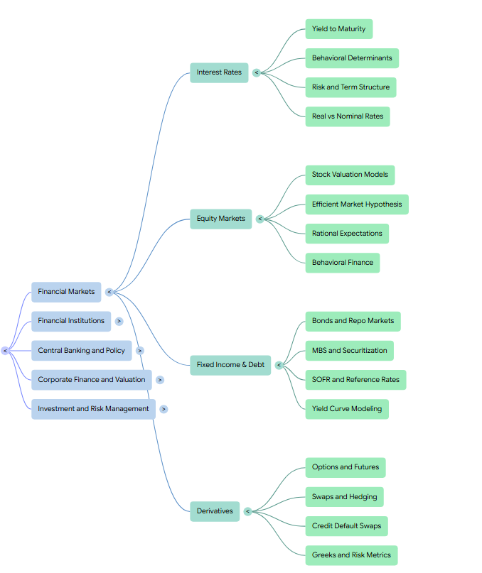
— Linden Lake

This series:
→　Domain Overview (1 of 5): Financial Markets
→　Domain Overview (2 of 5): Financial Institutions
→　Domain Overview (3 of 5): Central Banking and Policy
→　Domain Overview (4 of 5): Corporate Finance and Valuation
→　Domain Overview (5 of 5): Investment and Risk Management
→　Domain Mapping Methodology