Topic Review (7 of 7): Fixed Income – Quantitative and Statistical Techniques

Prior to the 1980s, fixed-income analysis was relatively straightforward, relying primarily on simple calculations of yield to maturity (YTM) and yield to call under passive, buy-and-hold strategies. However, as the debt markets expanded to include highly complex securities—such as non-investment-grade “junk” bonds, mortgage-backed securities (MBS), and debt with embedded options—practitioners recognized that simple yield-to-maturity metrics failed to capture key pricing and risk dynamics.

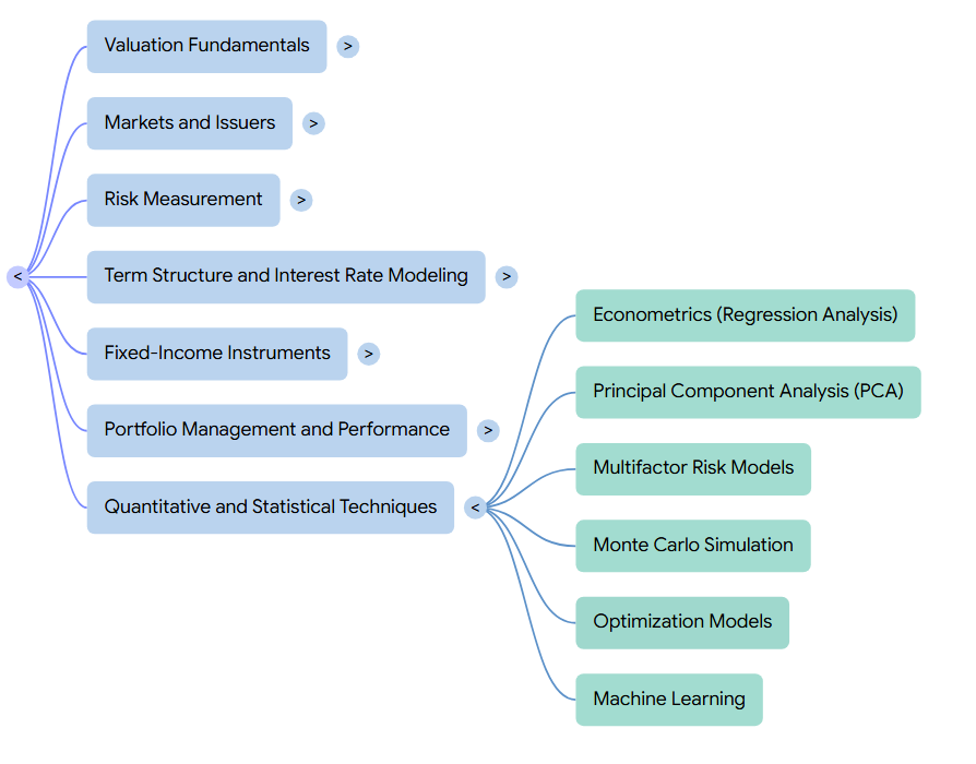
Modern active bond portfolio management requires a quantitative approach drawing heavily on statistics, financial econometrics, operations research, and data science. The sources outline several major quantitative and statistical frameworks that define modern fixed-income mathematics:

1. Advanced Regression Modeling and Empirical Risk Metrics

Linear regression is the foundational workhorse of financial econometrics, used to identify relationships among interest rates, economic factors, and bond prices.

Empirical Duration vs. Model Duration: While traditional “model” (or analytical) duration is calculated using theoretical prices derived from mathematical models when interest rates are shocked, empirical duration uses regression analysis on historical price and yield data to estimate interest rate sensitivity. The regression model is estimated as:

Change in Bond Price = a + b × (Change in Relevant Yield) + e

The estimated slope (b) is then divided by the bond’s full price to determine its empirical duration. Empirically, lower-credit-rated bonds (like high-yield debt) exhibit much lower empirical durations than analytical model durations. This occurs because credit risk, default risk, and credit-spread volatility have a much stronger influence on junk bond pricing than benchmark interest rate movements, which can be quantified by adjusting analytical duration with correlation-adjusted duration multipliers.

Regression-Based Hedging: Regression is extensively utilized to design optimal hedges. For instance, a market maker holding a non-Treasury bond can regress its yield changes against changes in a benchmark Treasury yield to compute a beta ( $\hat{\beta}$ ). This beta serves as a hedge ratio adjustment, minimizing the variance of the overall hedged portfolio’s profit and loss (P&L).

2. Multi-Factor Risk Decomposition and Principal Component Analysis (PCA)

Traditional interest rate sensitivity metrics (duration and convexity) assume a parallel shift in the yield curve, which rarely occurs in practice. To manage “shaping risk” (sensitivity to nonparallel twists and slope changes), quantitative analysts rely on multi-factor frameworks.

The Big Three Yield Curve Factors: Using Principal Component Analysis (PCA)—a non-parametric, statistical technique that extracts independent, uncorrelated factors from a historical variance-covariance matrix of rate changes—researchers have shown that 97% to 99% of yield curve volatility is explained by just three factors:
1. Level: Representing a parallel shift in the yield curve (accounting for roughly 77% to 92% of yield curve variation).
2. Slope (Steepness): Characterizing non-parallel shifts where short-term and long-term rates move differently (accounting for about 5% to 17% of variation).
3. Curvature (Twist): Depicting movements where short-term and long-term rates rise while intermediate rates fall, or vice versa (accounting for about 1% to 3% of variation).
Systematic Portfolio Construction: By mapping a portfolio’s sensitivities (factor loadings) to these principal components, managers can build precise hedges that neutralize specific yield curve reshaping risks, or construct highly optimized tracking portfolios that replicate benchmark indices while minimizing predictive tracking error.

3. Stochastic Modeling and No-Arbitrage Lattices

Fixed-income securities with path-dependent cash flows or embedded options (such as callable bonds, putable bonds, capped/floored floaters, and mortgage-backed securities) cannot be valued using a single static discount rate. They require a stochastic interest-rate model, which provides a probabilistic description of how interest rates vary randomly over time.

Equilibrium vs. No-Arbitrage Models: Equilibrium models (such as the Cox-Ingersoll-Ross [CIR] and Vasicek models) use economic variables to derive interest rate dynamics. While mathematically rigorous, they do not price standard benchmark bonds exactly. Conversely, no-arbitrage (arbitrage-free) models (such as the Ho-Lee, Kalotay-Williams-Fabozzi [KWF], and Black-Derman-Toy [BDT] models) calibrate their parameters to the current market term structure so that the model matches observed benchmark bond prices exactly.
Lattice Implementation: These models are implemented numerically using binomial and trinomial interest-rate lattices. To prevent the modeling of unrealistic negative interest rates (at least prior to the negative rate environments in Europe and Japan) and to capture higher volatility at higher rates, practitioners typically utilize lognormal random walks. Backward induction is then applied from right to left across the tree to calculate the fair option-adjusted values and effective durations of the option-contingent cash flows.

4. Quantitative Credit and Bankruptcy Prediction Models

To manage credit risk, quantitative techniques have replaced or heavily supplemented subjective human credit judgments.

Traditional Statistical Classifications: Analysts rely on statistical credit-scoring models to rank default probability. Multiple Discriminant Analysis (MDA), famously deployed in Edward Altman’s Z-score and Zeta models, simultaneously evaluates a large vector of financial accounting ratios to classify corporate borrowers into high- and low-default-risk groups.
Probability of Default (PD) Estimation: Rather than just classifying risk, linear probability models, logit models, and probit models are used to calculate the exact mathematical probability of default. Reduced-form models routinely apply logistic regressions to estimate how historical company-specific (leverage, equity volatility, excess returns) and macroeconomic variables (VIX, unemployment) drive default intensity over time.
Structural Option Models: Pioneered by Black, Scholes, and Merton, structural (firm-value) models treat a company’s equity as a European call option on the company’s underlying assets, with a strike price equal to the face value of its outstanding debt. The probability of default is then mathematically modeled as the probability that the company’s unobservable asset value falls below the default point at the debt’s maturity.

5. Operations Research: Monte Carlo Simulation and Optimization

Complex portfolios require sophisticated optimization and simulation tools to align portfolio assets with liabilities or indices under uncertainty.

Monte Carlo Simulation: When cash flows are highly path-dependent—such as mortgage-backed securities where a homeowner’s decision to prepay (refinance) is influenced by the historical trajectory of interest rates—analytical lattices fail because they have no “memory”. Analysts deploy Monte Carlo simulation to randomly generate thousands of arbitrage-free interest-rate paths, project mortgage prepayment speeds along each path, and average the discounted cash flows to calculate the security’s theoretical value and effective duration.
Optimization Models: Operations research provides several mathematical programming models to construct optimal portfolios:
- Linear Programming: Used in cash flow matching to minimize the initial cost of a portfolio subject to satisfying a strict multi-period liability schedule.
- Quadratic Programming: Deployed in index tracking and mean-variance asset allocation to minimize tracking error (or portfolio variance) subject to credit and sector guidelines.
- Mixed-Integer Programming: Crucial in real-world bond markets because bonds trade in round-lot sizes. It restricts decision variables to integer values to prevent the model from recommending un-tradeable fractional “odd-lot” transaction sizes.
- Robust Optimization: Modern portfolio theory is highly sensitive to estimation error in expected returns. Robust optimization replaces precise point estimates with defined “uncertainty sets” (such as confidence intervals around forecasts) to construct portfolios that remain stable even if market realizations deviate from the original forecasts.

Econometrics (Regression Analysis)

Foundations of Financial Econometrics and the Linear Regression Model

Financial econometrics is a specialized branch of economics that draws heavily on statistical techniques to model, test, and forecast financial relationships. It focuses on the mathematical representation and prediction of financial variables—such as asset prices, security returns, interest rates, default probabilities, recovery rates, and risk exposures.

The primary, most versatile tool in the financial econometrics toolkit is the linear regression model, which is used to estimate and quantify the structural relationship between a dependent variable and one or more independent (explanatory) variables.

Mechanics of Regression: Estimation and the Method of Least Squares

In its simplest form, a simple linear (univariate) regression model assumes a linear relationship between a dependent variable (Y) and a single independent variable (X), augmented by a random error term (e) to capture unexplained market noise:

Y = b₀ + b₁X + e

In this model, represents the intercept term, and represents the slope coefficient. Because financial relationships are estimated over time, this is typically formulated as a time-series regression model:

Y_t = b₀ + b₁X_t + e_t

To find the optimal values for the parameters and , econometrics relies on the Method of Least Squares (also called ordinary least squares, or OLS). Under this mathematical criterion, the parameters are chosen to minimize the sum of the squared differences (residuals) between the actual observed values of the dependent variable (Y_t) and the estimated values ( $\hat{Y}_t$ ) predicted by the regression line:

Squaring the errors ensures that positive and negative deviations do not artificially offset each other, while heavily penalizing larger, more extreme prediction errors. When these OLS assumptions are satisfied, the resulting parameter estimators are linear, unbiased, consistent, and efficient.

When a dependent variable is driven by more than one market factor, the model is expanded into a multiple linear regression model:

Y=b₀ + b₁X₁ + b₂X₂ + ⋯ + b_KX_K + e

In addition to quantitative variables, multiple regressions can incorporate qualitative (binary or dummy) variables. A dummy variable takes on a value of 1 if a specific qualitative attribute is present (e.g., a period of economic recession or a particular corporate sector) and 0 otherwise, allowing qualitative features to shift the intercept of the regression [228n20, 231, 369, 370].

Assessing Model Quality, Complexity, and Parsimony

Once a regression model is estimated, its explanatory power and predictive capability must be evaluated:

Coefficient of Determination (R²): This statistic measures the “goodness of fit” of the model, representing the percentage of the total variation in the dependent variable explained by the independent variables. It ranges from 0 to 1. In a single-variable regression, R² is exactly equal to the square of the correlation coefficient (r), which measures the statistical association between the two variables.
Standard Error of the Estimate (σ_ϵ): This represents the standard deviation of the regression residuals. It quantifies the remaining scatter of data points around the regression line and is used to compute confidence intervals for forecasted values.
The Adjusted R² and Parsimony: A major hazard in multiple regression modeling is overfitting. A model’s raw R² can be artificially inflated simply by adding more explanatory variables, but this often captures sample-specific noise, making the model overly complex, inflexible, and poor at out-of-sample forecasting. To penalize the excessive use of independent variables, analysts use the adjusted R², which accounts for both the number of observations and the number of parameters estimated. Econometricians aim to keep models as parsimonious as possible—using the fewest independent variables necessary to achieve maximum explanatory power.
Information Criteria (AIC and BIC): During the model selection stage, researchers compare candidate models using information-theoretic criteria that measure the expected loss of information. The Akaike Information Criterion (AIC) and the Bayesian Information Criterion (BIC) (also called the Schwartz Bayesian criterion) score candidate models by rewarding goodness of fit (log-likelihood) and penalizing the number of parameters [394, 395, 397n5]. The model with the lowest AIC or BIC score represents the optimal, most parsimonious fit. Notably, the BIC imposes a stricter mathematical penalty on the number of parameters than the AIC.

Diagnostic Testing: Verifying Assumptions and Remedying Violations

To ensure that OLS parameter estimates and their associated statistical significance tests (such as the Studen t -test and F -test) are valid, the model must undergo rigorous diagnostic testing to check for violations of core econometric assumptions:

1. Multicollinearity

This violation occurs when two or more independent variables in a multiple regression are highly correlated with each other, meaning they contain overlapping information. While the overall model may still appear highly significant, multicollinearity inflates the standard errors of the regression coefficients, making it difficult to isolate the true individual impact of each explanatory variable.

Detection: Analysts review pairwise correlation matrices and calculate the Variance Inflation Factor (VIF), which measures how much the variance of an estimated coefficient is inflated. A VIF of 1 indicates no correlation, a VIF between 1 and 5 indicates moderate correlation, and a VIF exceeding 5 indicates high multicollinearity, requiring the removal or consolidation of the redundant independent variables.

2. Heteroscedasticity

The classical OLS model assumes homoscedasticity, meaning the variance of the probability distribution of the error term is constant across all observations. When this assumption is violated, the error terms are heteroscedastic, meaning their variances vary (e.g., they are systematically larger for some periods or levels of the independent variables than others), which is very common in financial time series.

Remedy: If heteroscedasticity is detected, standard coefficient standard errors are biased. Analysts must utilize either the weighted-least-squares (WLS) estimation technique or AutoRegressive Conditional Heteroscedasticity (ARCH) models, which explicitly model and forecast the time-varying variance of the error term.

3. Autocorrelation (Serial Correlation)

OLS assumes that the error terms are completely uncorrelated from one observation to the next. If error terms are correlated across consecutive periods (common in time-series data), they are autocorrelated, exhibiting persistence (positive autocorrelation) or systemic reversal (negative autocorrelation). Autocorrelation severely understates the standard errors of the regression coefficients, leading to inflated, misleadingly significant -statistics.

Detection & Remedy: Autocorrelation is diagnosed using the Durbin-Watson (d) test or the Dickey-Fuller test. For the Durbin-Watson statistic, a value near 2 indicates no autocorrelation, a value near 4 indicates negative autocorrelation, and a value near 0 indicates positive autocorrelation. To correct for autocorrelation, analysts implement AutoRegressive Moving Average (ARMA) models.

The Three-Step Financial Modeling Process

Applying regression analysis systematically within fixed income involves three consecutive, formalized stages:

Model Selection: Justifying a family of models on the basis of sound economic intuition and financial theory. Econometricians must avoid blind data mining (letting flexible models fit any dataset purely statistically), as it risks capturing sample-specific noise that will fail out-of-sample.
Model Estimation: Linking mathematical models to financial reality by using historical sample data to estimate the optimal model parameters via methods like Least Squares, Maximum Likelihood, the Method of Moments, or Bayesian methods.
Model Testing (Backtesting): Validating the estimated model on out-of-sample data (data completely separate from the training set used to fit the model) to ensure it did not capture historical anomalies.

Critical Applications of Regression in Fixed Income

The sources detail several prominent areas where regression analysis is indispensable to bond portfolio management and market design:

A. Empirical Duration

While theoretical “model” durations are derived analytically from pricing formulas under yield-shock assumptions, empirical duration uses regression analysis on historical price and yield data to measure actual market price sensitivity. Econometricians estimate the following simple linear regression:

Change in security’s price = a + b(change in relevant yield)

Dividing the estimated slope (b^) by the security’s full price yields its empirical duration. Empirical duration is highly valuable because it does not rely on restrictive theoretical assumptions and is simple to compute. It frequently reveals that lower-rated corporate bonds (high-yield “junk” bonds) have significantly lower empirical durations than analytical modified durations. This occurs because credit risk, default risk, and spread volatility dominate corporate bond pricing over Treasury interest-rate changes.

To bridge this gap, Barclays researchers developed duration multipliers (M) to scale down model duration (D) using the historical correlation and standard deviation of Treasury yield changes relative to corporate credit-spread changes:

Empirical Duration = M ×D

B. Returns-Based Style Analysis (RBSA)

Developed by William Sharpe, RBSA is a low-cost, statistically driven alternative to holdings-based performance attribution. It does not require proprietary, security-level holdings. Instead, RBSA runs a multiple linear regression where historical portfolio returns are the dependent variable and the historical returns of passive, liquid strategy index factors (such as bond trend, bond carry, FX volatility, FX carry, and rate volatility) are the independent variables.

The model solves for the beta exposures (β_i ) of each factor subject to the strict constraint that the sum of the estimated betas must equal 1 (∑β_i=1). To capture how a manager’s active allocation style dynamically shifts over time, analysts execute rolling style analysis using short, moving windows (e.g., 26 weeks).

C. Regression Hedging and P&L Variance Minimization

In the cash and derivatives markets, OLS is used to construct optimal risk hedges. A market maker holding a bond to be hedged can regress its daily yield changes against the daily yield changes of a hedging instrument (such as a liquid Treasury or the cheapest-to-deliver bond futures contract) to estimate a slope coefficient ( $\hat{\beta}$ , or yield beta). This yield beta acts as the optimal hedge ratio (risk weight):

By choosing this specific hedge ratio, the variance of the overall hedged portfolio’s P&L is mathematically minimized. The standard deviation of the resulting hedged P&L is simply the product of the asset’s DV01 and the standard error of the regression residuals (σ_ϵ).

When setting up these hedges, practitioners must make critical modeling decisions:

Level vs. Change Regressions: Regressing yields on yields (level regressions) typically violates the assumption of error independence, exhibiting highly persistent serial correlation. Regressing changes in yields on changes in yields (change regressions) is the industry standard because it models daily price fluctuations more realistically, though any remaining serial correlation must be handled using autoregressive error models (ϵ_t =ρϵ _t−1+v_t ).
Reverse Regressions: Regressing the hedging instrument on the asset instead of the asset on the hedging instrument yields different slope coefficients. The choice depends on the trader’s core objective (e.g., minimizing the variance of a fixed-size asset position versus a fixed-size hedging instrument).

D. Relative-Value Yield Curve Fitting

To execute relative-value trades, analysts construct a benchmark “fair-value yield curve” across the term structure by applying cross-sectional regressions to a reference set of liquid default-free bonds. Individual bonds are then mapped against this baseline: bonds trading at yields above the regression-fitted curve are labeled “cheap” (undervalued), while bonds trading below are labeled “rich” (overvalued). To measure the statistical significance of these deviations, quantitative platforms calculate a bond’s Z-score (the number of standard deviations the current yield is from the historical mean), trading on the expectation that extreme Z-scores will mean-revert to the fitted baseline.

E. Corporate Credit and Bankruptcy Prediction

In credit risk management, regressions are used to model default probability and loss severity:

Multiple Discriminant Analysis (MDA): Altman’s Z-score and Zeta models use MDA to simultaneously analyze a vector of accounting ratios (e.g., leverage, EBIT/assets, liquidity) to classify corporate borrowers into distinct high- and low-default-risk groups.
Linear Probability Models: These utilize standard multiple linear regression (OLS) where the dependent variable is a binary default flag (1 for default, 0 for survival). A major drawback is that the predicted default probability can be negative or exceed 1.
Probit and Logit Regression Models: To force the predicted default probability strictly between 0 and 1, credit models apply these non-linear regressions. A probit model restricts predictions to a standard normal cumulative probability distribution (N(W)), while a logit model restricts predictions to the cumulative distribution of a logistic distribution (1/(1+e^−W)).

F. Liquidity Cost Scores (LCS)

Because thousands of corporate bonds do not trade actively on a daily basis, real-time liquidity quotes are scarce. To estimate a bond’s Liquidity Cost Score (LCS)—which represents its estimated bid-ask spread as a percent of price—analysts run a cross-sectional multiple linear regression. By regressing observed, reliable bid-ask quotes of actively traded bonds against their observable attributes (such as issue age, monthly trading volume, issuer size, credit rating, sector, and duration times spread [DTS]), the model estimates a statistical relationship that is then applied to calculate the implied LCS for unquoted, illiquid bonds.

Principal Component Analysis (PCA)

Core Concepts and Mathematical Structure

In the framework of quantitative fixed-income analysis, Principal Component Analysis (PCA) is a powerful statistical tool used to parsimoniously represent large datasets. Rather than analyzing dozens of correlated variables individually, PCA transforms a large number of explanatory variables into a much smaller set of uncorrelated, synthetic variables called principal components (PCs) or factors, which are linear combinations of the original variables.

Mathematically, a principal component (Fj) is formulated as:

F_j=c_j1X₁+c_j2X₂+⋯+c_jKX_K

where represents the original explanatory variables (such as individual interest rates or yields along the curve), and the coefficients are estimated by the PCA and referred to as the factor loadings.

Within fixed-income portfolio management, PCA is most commonly applied to explain the daily fluctuations and risk dynamics of the yield curve, as well as to identify broader systematic risk factors across different bond portfolios.

The Three Key Properties of Principal Components

When constructing PCs from a variance-covariance matrix of interest rate movements, the mathematical optimization ensures that the factors satisfy three essential properties:

Total Variance Conservation: The sum of the variances of the individual principal components is exactly equal to the sum of the variances of the individual underlying rates.
Orthogonality: The principal components are constructed to be completely uncorrelated (orthogonal) with one another, even though the original interest rates are highly intercorrelated.
Sequential Variance Maximization: Each PC is sequentially chosen to capture the maximum possible variance remaining after the prior PCs have been extracted. Consequently, the first PC has the largest explanatory power, the second PC has the second-largest, and so on.

Yield Curve Dynamics: Level, Slope, and Curvature

Empirical studies globally demonstrate that the vast majority of yield curve movements can be captured by just a few principal components. Historically, Litterman and Scheinkman established that three factors explain the returns of Treasury portfolios. These are economically interpreted as Level, Slope, and Curvature:

The Level Factor (PC1): This component represents a roughly parallel shift across the entire length of the yield curve. It is by far the most dominant factor, typically explaining 90% to 92% of the total variance across all rates. For example, in a study of USD LIBOR swap rates, a one standard deviation positive move in the level factor was shown to shift the 1-year rate up by 0.23 basis points, the 10-year up by 3.44 basis points, and the 30-year up by 3.77 basis points.
The Slope Factor (PC2): This component represents a non-parallel shift where short-term and long-term rates move in opposite directions, altering the steepness of the curve. It typically accounts for 5% to 8% of the total variance. A positive standard deviation change in the USD LIBOR slope factor causes the 1-year and 2-year rates to fall (by 0.16 and 0.51 bps respectively) while the 10-year and 30-year rates increase (by 0.07 and 1.35 bps).
The Curvature Factor (PC3): This component represents a “hump” or “twist” in the curve, where short- and long-term rates move in one direction while intermediate-term rates move in the opposite direction. It explains roughly 1% to 3% of the variance. This factor is highly useful for explaining localized variation in short-term rates.
The “Snake Shift” (PC4): Some long-term historical studies (e.g., U.S. Treasury yields from 1984 to 2020) identify a highly minor fourth PC explaining about 0.5% of the variance, which has less economic intuition and is referred to as a “snake shift”.

Together, these first three principal components explain over 99% of the variation for all yields of maturities greater than three years.

International Comparisons and Macro Volatilities

The structure and explanatory power of principal components exhibit distinct variations across different global sovereign debt markets:

Parallel Shift Dominance: In a comparative study of government bond maturities across different nations, the first PC (level shift) was found to be less dominant in Canada, the United Kingdom, Germany, and Japan relative to the United States. This carries the major risk-management implication that traditional, single-factor duration (which assumes parallel shifts) is a poorer measure of interest rate sensitivity in those countries than it is in the US.
Volatility Magnitudes: Comparing USD, GBP, and EUR swap rates, the shapes of the PCs are qualitatively similar, but the volatility of Euribor swap rates is significantly lower than its USD and GBP counterparts. For instance, while the USD and GBP level PCs flatten out at over 3.5 basis points per day in the long end, the EUR level PC flattens out at just above 2.5 basis points. This is attributed to the aggressive monetary policy of the European Central Bank to keep short-term interest rates low over an extended period.

Applications to Hedging and Portfolio Management

Using PCA in portfolio construction and risk management provides significant advantages over traditional yield-based metrics:

1. Robust Multi-Factor Hedging

To construct a hedge with PCA, a manager calculates the current portfolio price, shifts the term structure by each PC, determines the portfolio’s sensitivity (’01) to each PC, and subsequently selects a set of hedging securities to neutralize these specific PC exposures. Axel and Vankudre demonstrated that PCA-based hedges are highly superior to traditional duration-neutral hedges, resulting in significantly lower out-of-sample profit-and-loss (P&L) variance.

2. Sizing Complex Relative-Value Trades

For a multi-rate relative value trade (such as a 10s-20s-30s butterfly swap), a trader can neutralize level and slope risks using PCA. For example, in a USD swap butterfly where the trader is receiving fixed in the 20-year swap, PCA-implied risk equations dictate shorting 10-year and 30-year swaps.

The resulting risk weights are 27.1% in the 10-year swap and 74.1% in the 30-year swap. Because the 10-year swap is significantly less sensitive to level and slope shifts, more overall DV01 risk is required in the hedge, causing the total risk weights to sum to 101.2% rather than the 100% implied by simple parallel-shift assumptions.

3. Defining Strategic Factor Requirements

PCA helps managers determine how many risk factors must be neutralized depending on the maturity sector they trade. Because the level PC dominates the middle of the curve, traders operating strictly in the 8-to-10-year swap range can safely defend using a simple one-factor model. However, traders active in the 3-to-6-year sector, the long end, or the very short end require more robust two-factor or three-factor models to handle shaping and curvature risks.

Identifying Broader Bond Risk Factors

Beyond yield curve term structures, PCA is utilized to extract non-term risk factors by analyzing historical excess bond returns alongside macroeconomic and market variables. For example, Gauthier and Goodman applied PCA to the nominal excess returns of the Salomon Smith Barney Broad Investment Grade (SSB BIG) Index and identified three principal components explaining 98.1% of the total return variation:

Factor 1 (The Interest Rate/Term Factor): Explaining 92.7% of the variation, this PC has factor loadings that track the average duration of each bond sector and exhibits a clear linear correlation with changes in the 10-year Treasury yield.
Factor 2 (The Credit Factor): Explaining 3.1% of the variation, this factor has high negative loadings on corporate credit and high positive loadings on Treasury bonds. It has a -0.5 correlation with the S&P 500 Index, reflecting that lower equity market performance correlates directly with lower corporate bond returns.
Factor 3 (The Optionality Factor): Explaining 2.3% of the variation, this PC has positive loadings on asset classes with embedded options (such as MBS, ABS, and callable agencies) and negative loadings on noncallable bonds. It is positively correlated with the slope of the yield curve and negatively correlated with short-term interest rate volatility (5-year cap volatility).

Multifactor Risk Models

Modern active bond portfolio management has transitioned away from a historical reliance on simple, static measures—such as yield to maturity (YTM) or rating-agency classifications—toward sophisticated multifactor risk models . In actively traded fixed-income markets, these models draw heavily on statistics, financial econometrics, operations research, and data science to systematically decompose, monitor, and construct portfolios relative to a designated market benchmark .

1. Decomposing Fixed-Income Risk via Multifactor Models

Multifactor risk models systematically isolate and categorize risk exposures into distinct systematic and nonsystematic components :

Systematic Risk: The risk inherent in the entire market or a broad segment . Systematic risk is divided into two primary subcategories:
- Term-Structure Risks: Risks associated with shifts in the level and shape (slope and curvature) of interest rate and credit spread curves . Portfolio sensitivity is quantified using measures like modified duration, effective duration, and key rate durations .
- Non-Term-Structure Risks: Risks that capture yield-spread volatility across various non-interest-rate dimensions, including sector exposures (industry groups), quality exposures (credit ratings and defaults), coupon structures, and optionality/vega (interest-rate volatility) .
Nonsystematic (Idiosyncratic) Risk: Risk associated with exposures to particular corporate issuers or specific issues . Unlike systematic factors, idiosyncratic risks represent localized exposures (such as credit default or downgrade risk of a specific name) that can be mitigated through broad portfolio diversification .

Prominent Model Architectures

In institutional practice, leading asset managers and analytics groups utilize specialized models with distinct factor structures:

The Axioma Fixed-Income Risk Model: Categorizes systematic risk factors into Rates (zero-rate curves, swap-spread curves, inflation curves, and spot FX), Credit Spreads (OAS decomposed into cross-sectional sector, country, quality, and market factors), MBS Spreads (decomposed into pool-level spread, refinance, and turnover risks), and Volatility (swaption and equity implied volatility surfaces) .
Amundi Asset Management’s Risk Model: Separates risk factors into systematic term-structure elements (duration and credit risk), systematic non-term-structure elements (sector, quality, optionality, and coupon risks), and nonsystematic issuer- and issue-specific risks .

2. The Core Metric: Forward-Looking Tracking Error

In multifactor risk models, the principal metric used to manage and control active portfolio risk relative to a benchmark is forward-looking (predictive) tracking error . This metric represents the annualized predicted standard deviation of the active return (the portfolio’s return minus the benchmark’s return) .

Mathematical Aggregation of Risk Factors

To calculate a portfolio’s total systematic tracking error, the individual isolated risk factor exposures must be mathematically aggregated:

Orthogonal (Uncorrelated) Factors: If the risk factors are statistically independent, the portfolio’s isolated systematic tracking error is computed as the square root of the sum of the squared individual tracking errors:

Correlated Factors: When risk factors exhibit non-zero correlations, the modeler must utilize the variance-covariance matrix of the factors to capture pairwise covariances:

Risk Allocation and Sensitivity Metrics

Multifactor risk models provide portfolio managers with advanced diagnostic metrics to analyze active risk positioning:

Idiosyncratic Tracking Error and Name Risk: In portfolios with a restricted number of holdings, idiosyncratic risk heavily dominates the active tracking error (even when systematic risk explains over 99% of the absolute standard deviation of the returns) . This exposes the portfolio to severe name risk (unhedged single-issuer concentration) .
Liquidation Effect: This represents the change in the portfolio’s total tracking error that would result from completely hedging or eliminating exposure to a specific risk factor group or asset class .
Factor Betas: A beta-type measure calculated for individual risk factors to evaluate portfolio-level sensitivity relative to the benchmark (e.g., a duration beta equals portfolio duration divided by benchmark duration) .
Return Impact of Typical Movements: Estimates the isolated return change of the portfolio relative to the benchmark from a typical one standard deviation move in a factor, computed as:

Return Impact = −(net factor exposure) × typical factor volatility

3. Integration with Broader Quantitative and Statistical Techniques

Multifactor risk models are not isolated frameworks; they represent the convergence of several foundational mathematical and statistical disciplines :

A. Econometrics & Machine Learning (LASSO & VIF)

To prevent overfitting when managing portfolios with hundreds of potential factors, modern risk engines employ regularized regression and machine learning algorithms .

Amundi’s LASSO Factor Picking: The Amundi model utilizes the Least Absolute Shrinkage and Selection Operator (LASSO) regression technique . LASSO performs both parameter shrinkage and variable selection by forcing less informative coefficients to zero, allowing the model to systematically identify and rank the most pertinent risk factors (empirically isolating issue-specific and issuer-specific factors as the dominant drivers of active return variance) .
Variance Inflation Factors (VIF): To ensure OLS or machine-learning regressions are statistically stable and robust, analysts compute VIFs to check for multicollinearity . A VIF value below 5 confirms low linear dependence among the chosen risk factors, ensuring that the estimated risk parameters do not fluctuate wildly due to minor changes in market data .

B. Principal Component Analysis (PCA)

Rather than analyzing dozens of highly correlated yields along a curve, quantitative frameworks rely on Principal Component Analysis (PCA) to parsimoniously represent yield curve dynamics . PCA extracts uncorrelated (orthogonal) factors from a historical variance-covariance matrix of rate changes :

Level (PC1): Captures a parallel shift across the yield curve, explaining approximately 90% to 92% of overall curve variance .
Slope (PC2): Captures a non-parallel flattening or steepening of the curve, explaining roughly 5% of variance .
Curvature (PC3): Captures a non-parallel “twist” or “hump” in the curve, explaining about 1% to 3% of the variance .

Fixed-income managers map their portfolio exposures directly to these orthogonal PCs to construct highly robust multi-factor hedges that neutralize nonparallel shaping and curvature risks, outperforming traditional duration-neutral hedges .

C. Constrained Optimization Models

To build or rebalance portfolios, multifactor risk models are paired with mathematical optimizers .

The Objective Function: The optimizer’s mathematical objective is to find the exact weight of each bond to hold in order to minimize the portfolio’s forward-looking tracking error relative to a benchmark .
Imposing Constraints: This minimization is solved subject to strict constraints, such as matching key rate durations, sector/quality weights, currency exposures, and maximum individual issuer concentrations .
Mixed-Integer Programming: Because bonds trade in round lots, optimizers use mixed-integer linear and quadratic programming to restrict purchase decision variables to integer values, preventing the model from recommending un-tradeable fractional “odd-lot” transaction sizes .

D. Monte Carlo Simulation

While standard binomial or trinomial interest-rate lattices are highly efficient for path-independent options (where cash flows do not depend on how interest rates arrived at a specific node), they fail to accommodate path-dependent cash flows .

In Mortgage-Backed Securities (MBS), prepayments are highly path-dependent due to “prepayment burnout” (where past interest rate trajectories permanently alter current homeowner refinancing behavior) .
To value these assets, quantitative managers deploy Monte Carlo simulation to generate thousands of randomized, random-walk interest-rate paths . The paths are calibrated to today’s risk-free spot curve to ensure they are arbitrage-free , allowing the model to accurately project expected prepayment cash flows and compute effective duration and effective convexity .

Monte Carlo Simulation

Monte Carlo simulation is a foundational operations research and management science tool used when the outcome of a decision depends on several highly complex, random variables. While traditional financial econometrics—such as linear regression—has historically been the workhorse for identifying market patterns, it assumes rigid linear relationships. In contrast, Monte Carlo simulation provides fixed-income portfolio managers, analysts, and traders with the mathematical flexibility to model nonlinear, multi-variable, and path-dependent systems under extreme uncertainty.

1. The Path-Dependency Mandate: Lattices vs. Simulation

In fixed-income mathematics, a core distinction is made between securities whose cash flows are interest-rate-path-independent versus interest-rate-path-dependent. This distinction dictates whether an analyst can use a simple lattice (tree) or must deploy a Monte Carlo simulation:

Path-Independent Cash Flows (Lattice Models): For instruments like standard callable, putable, or municipal bonds, the cash flows at any given node of a binomial or trinomial interest rate tree depend only on the interest rate at that specific node. How the interest rate arrived at that node is irrelevant. Thus, backward induction on a closed-form lattice is the preferred, computationally efficient choice.
Path-Dependent Cash Flows (Monte Carlo Simulation): For securitized products like Residential Mortgage-Backed Securities (RMBS) and Collateralized Mortgage Obligations (CMOs), cash flows are heavily path-dependent due to the phenomenon of prepayment burnout. Homeowners do not prepay mortgages based solely on current interest rates; their propensity to refinance is heavily influenced by the historical trajectory of interest rates. Because traditional lattices do not possess “memory” of past nodes, they cannot naturally accommodate this path-dependency. Consequently, portfolio managers must utilize Monte Carlo simulation to project thousands of individual interest rate paths and model cash flows dynamically along each unique timeline.

2. Arbitrage-Free Path Generation and Model Plumbing

To value a path-dependent security, a Monte Carlo model must simulate future interest rate paths using a mathematically rigorous, structurally sound framework:

Generating the Paths: The simulation takes today’s term structure (typically the Treasury spot-rate curve or a benchmark like SOFR) and an interest-rate volatility assumption as inputs. The volatility parameter determines the statistical dispersion of future rates.
Arbitrage-Free Calibration (Drift Adjustment): To ensure the model is “fair” and consistent with the law of one price, it must be calibrated so that the average simulated price of a zero-coupon benchmark Treasury bond across all paths exactly equals its actual market price. Since standard random-rate generators will not achieve this by chance, a mathematical drift-adjustment term (a constant) is added to the short-rate-generating process across all paths.
Mean Reversion: To prevent simulated interest rates from drifting into unrealistic extremes (such as or ) over a 30-year horizon, models incorporate mean reversion. This constraint pulls interest rates back toward the long-term implied forward rates derived from the initial yield curve.
Variance Reduction & Standard Error: In a statistical sampling process like Monte Carlo, increasing the number of simulated paths increases the precision of the estimated value by reducing the mean standard error. Because generating thousands of paths is computationally expensive, practitioners deploy variance-reduction techniques (such as the antithetic and control variates methods) to obtain highly precise estimates “within a tick” using fewer paths.

3. Advanced Applications: Credit Risk, OAS, and Risk Distribution

Beyond mortgage prepayment modeling, Monte Carlo simulation is heavily integrated into several key quantitative and statistical areas:

Option-Adjusted Spread (OAS): In the Monte Carlo framework, the OAS is the constant spread (K) that must be added to all spot rates along all simulated paths to equate the average present value of those paths to the security’s observed market price.
Decomposing Path Present Values: Traditionally, simulation models only report the average present value across all paths (the “theoretical value”). However, the sources emphasize that the probability distribution of path present values provides invaluable risk-management insights. For instance, a well-protected PAC (planned amortization class) bond will have a tightly concentrated distribution of path present values (a small standard deviation), whereas a highly volatile support CMO tranche will exhibit a wide, highly dispersed distribution (a large standard deviation).
Credit Portfolio Correlation Risk: Because corporate defaults are rare, historical default correlation data is scarce. To assess credit portfolio risk, risk managers use Monte Carlo simulation on historical rating changes and equity price correlations to model joint default events and quantify default dependencies across sectors.

4. Backtesting Systematic Investment Strategies

When developing systematic bond trading strategies, Monte Carlo simulation is mathematically superior to traditional historical backtesting methods:

Walk-Forward Limitations: The common walk-forward backtesting method assumes that history repeats itself along a single historical path. This fails to account for alternative market scenarios, can be heavily biased by a specific sequence of historical data, and fails to reveal why a strategy succeeded or failed.
The Simulation Advantage: Unlike walk-forward tests, Monte Carlo backtesting generates hundreds of out-of-sample randomized paths. This allows portfolio managers to conduct randomized, controlled experiments, analyze strategy performance under customized stress scenarios, incorporate event probabilities before new data is collected, and expand the length of the backtest arbitrarily to achieve a targeted statistical degree of confidence.
Biases to Watch: When implementing Monte Carlo backtests, modelers must actively guard against systematic biases. These include optimal-period bias (selecting favorable windows), time-period bias (date sensitivity), survivorship bias (using only currently surviving corporate entities, which artificially inflates historical returns), and look-ahead bias (using regulatory or financial data that was not yet publicly released at the simulated trade date).

Optimization Models

In the modern fixed-income landscape, optimization models are essential quantitative tools used to prescribe the best course of action to achieve a specific portfolio objective. Because fixed-income portfolios are actively traded and highly complex, managers have shifted away from simple buy-and-hold approaches toward these mathematical programming frameworks to systematically align assets with benchmarks, fund liabilities, and allocate capital.

1. Setting Up a Mathematical Programming Model

To construct any optimization model in fixed income, a practitioner must configure four fundamental mathematical steps:

Define the Decision Variables: These represent the actual choices to be made, typically the weight or par amount of each individual bond to buy or sell.
Specify the Objective Function: The mathematical formula the manager seeks to optimize—either minimizing an undesirable element (like transaction costs or tracking error) or maximizing a desirable one (such as expected return or convexity).
Establish the Constraints: These are the physical, regulatory, or client-mandated boundaries that the optimal solution must satisfy. Common constraints include risk budgets, duration matching, and maximum exposures to specific sectors, industries, or issuers.
Solve for the Optimal Solution: Numerical algorithms search through the set of feasible portfolios to identify the single portfolio that satisfies all constraints while maximizing or minimizing the objective function.

2. The Convex Optimization Hierarchy

Modern fixed-income optimization relies heavily on convex optimization problems. Unlike non-convex functions, which can trap a mathematical solver in sub-optimal local minima, a convex minimization problem possesses a unique global solution. Fixed-income applications primarily utilize three tiers of the convex optimization hierarchy:

A. Linear Programming (LP)

In an LP model, both the objective function and all constraints are strictly linear. The primary fixed-income application of LP is cash flow matching, where a manager seeks to build a minimum-cost portfolio of default-free bonds whose maturing principal and coupons match a scheduled liability stream.

B. Quadratic Programming (QP)

QP models permit a quadratic objective function while maintaining linear constraints. Since variance and standard deviation are quadratic terms (the weights are squared), QP is the mathematical engine of mean-variance asset allocation (minimizing portfolio variance for a target return) and index tracking/enhanced indexing (minimizing predicted tracking error relative to a benchmark index).

C. Second-Order Cone Programming (SOCP)

SOCPs represent a more advanced class of convex programming that minimizes a linear function subject to the intersection of second-order (quadratic) cones. This allows managers to incorporate curvature information directly into their risk-budgeting equations. SOCPs are heavily utilized in Conditional Value-at-Risk (CVaR) optimization to minimize expected tail loss across multiple risk factors, as well as in robust optimization formulations.

D. Mixed-Integer Programming (MIP)

Traditional LP and QP models assume decision variables are infinitely divisible. In the actual bond market, however, securities are traded in standard round-lot sizes. An unconstrained optimizer might suggest buying fractional “odd-lot” amounts, which are illiquid and expensive to execute. Mixed-integer programming solves this by restricting purchase variables to integer multiples of standard lot sizes.

3. Optimization Under Uncertainty

A primary challenge in quantitative finance is that model parameters (such as expected returns, volatilities, and correlations) are rarely known with certainty because they are estimated with error or represent future stochastic pathways. To address this estimation risk, fixed-income mathematics utilizes three distinct optimization-under-uncertainty frameworks:

Dynamic Programming: A sequential, multi-stage optimization method that solves complex problems by working backward from the final period to the present, maintaining the optimal path at each intermediate step.
Stochastic Programming: This framework models uncertainty using explicit probability distributions for future parameters. A key concept is recourse—the decision-maker’s ability to take corrective action in a subsequent stage after a random market event has occurred. Stochastic programming is widely applied to optimize mortgage-backed securities (MBS) portfolios, where future prepayments are highly uncertain and path-dependent.
Robust Optimization: Because probability distributions are themselves difficult to estimate accurately, classic stochastic programming can be computationally prohibitive and sensitive to error. Robust optimization replaces probability distributions with defined uncertainty sets (such as confidence intervals around expected return forecasts). The model optimizes for the worst-case scenario within those sets. Empirical testing indicates that robust optimization eliminates extreme “corner solutions” and generates significantly more stable portfolio weights over time, preserving the manager’s turnover and transaction cost budgets during rebalancing.

Machine Learning

Historically, financial econometric tools—particularly linear regression—have been the traditional workhorse for bond portfolio managers looking to identify pricing and risk patterns in historical data. However, Machine Learning (ML) is driving a paradigm shift by providing quantitative teams with modern, non-linear, and highly dimensional techniques to build predictive models that extract complex patterns.

This quantitative evolution is primarily a consequence of cheap, high-performance computing, which allows a family of highly flexible models to approximate sample data with virtually unlimited precision. While traditional econometric models are prone to misspecification and “false discoveries” (Type I and Type II errors) when failing to detect patterns, ML models automatically optimize a sequence of actions based on experience. Crucially, ML algorithms do not depend on specific financial theory; instead, they rely on purely statistical analysis of financial phenomena while imposing mathematical constraints on model complexity to preserve out-of-sample forecasting capabilities on unseen data.

1. The Financial Data Environment

A key strength of ML in fixed income is its ability to process a much wider array of data classes than traditional statistical tools. The sources segment these inputs along three distinct axes:

Quantitative vs. Qualitative: Quantitative data (such as historical returns, accounting ratios, or recovery rates) are numerical and can undergo direct mathematical transformations. Qualitative data (such as fixed-income sectors, credit rating categories, or whether a bond is callable) represent non-numerical attributes. They can be encoded numerically, but cannot undergo mathematical computations since they are merely labels.
Structured, Unstructured, and Semistructured: Structured data are objectively represented. Unstructured data (such as SEC filings, bond prospectuses, research reports, or even satellite images) lack a recognizable structure and are historically difficult to analyze. Semistructured data (like emails with attachments) fall in between. Modern fixed-income data science heavily leverages ML to extract actionable, structured information from unstructured and semistructured data.
Labeled vs. Unlabeled: Unlabeled data (such as transcripts of analyst webcasts, news articles, or tweets) lack identifying tags. Experts must perform the critical task of “labeling” or “tagging” this data (such as classifying the sentiment of a tweet). The sources note that ML does not eliminate human judgment; rather, human experts are indispensable because inaccuracies in labeling will directly compromise the integrity of the ML model.

2. The Four Machine Learning Architectures

Depending on the feedback and data provided to the algorithm during its training phase, ML models are categorized into four core architectures:

A. Supervised Learning

The algorithm trains on labeled data where the correct output (response variable) is paired with the input variables (features).

Regression ML: Used to predict a continuous numerical value. From a practical standpoint, there is no mathematical difference between regression ML and traditional financial econometrics; a bond manager using a regression ML algorithm to estimate the price sensitivity of a corporate bond to a Treasury rate shock is calculating empirical duration.
Classification ML: Establishes rules to assign inputs into discrete categories. An example is predicting whether a high-yield bond is a candidate to be upgraded, downgraded, or remain unchanged.
Key Algorithms: Supervised learning utilizes Decision Trees, Naive Bayes, Support Vector Machines (SVMs) (which synthesize features into a dividing hyperplane), Neural Networks (which mimic the human brain using input, hidden, and output layers with activation and loss functions), and Linear Regularization Models. Regularization models—specifically LASSO, Ridge, and Elastic Net—shrink regression coefficients to prevent overfitting. LASSO is highly favored because it shrinks uninformative coefficients completely to zero, performing automatic feature selection.
Ensembles: To decrease variance, reduce bias, or improve predictive power, managers combine multiple algorithms into “ensembles”. These include Bootstrap Aggregation (bagging)—which averages predictions across randomized data subsets with replacement (e.g., Random Forests)—and Boosting (such as AdaBoost), which iteratively converts “weak learners” into “strong learners”.

B. Unsupervised Learning

The algorithm is fed unlabeled data and must discover hidden groupings or structures based solely on the data’s statistical properties.

Key Algorithms: Principal Component Analysis (PCA) and Clustering Analysis (such as agglomerative/divisive hierarchical clustering or k-means clustering).
Fixed-Income Application: In k-means, data points are partitioned into clusters around centroids by minimizing the within-cluster sum of squares (WCSS), mapped via the “elbow method”. In the credit markets, clustering is highly valuable for marking-to-market illiquid debt instruments; the algorithm identifies actively traded bonds with highly similar statistical characteristics to price the illiquid issue.

C. Semisupervised Learning

Combines a small set of labeled data with a large set of unlabeled data to improve the learning behavior of supervised models when labeled data are scarce or too expensive to acquire.

D. Reinforcement Learning (RL)

Designed for interactive, dynamic systems (like the game of chess) where there is no static label. The algorithm chooses actions in an environment based on its current “state,” receiving feedback through a user-defined reward function. The goal is to maximize the cumulative reward over time, forcing the machine to selectively explore suboptimal paths to discover more profitable long-term strategies.

3. Critical Fixed-Income Applications

The integration of ML into fixed-income analysis has provided significant enhancements across several key operational areas:

Predicting CMBS Default Rates: Finding relative value in Commercial Mortgage-Backed Securities (CMBS) tranches requires predicting the default probabilities of the underlying commercial properties. While traditional models relied on logistic regression, modern studies demonstrate that ML classifiers—including SVM, random forest, and boosting—substantially outperform traditional benchmarks. SVM models are particularly effective because they allow an optimizer to attribute significance to multiple property-level financial metrics (such as debt-service coverage and loan-to-value ratios) simultaneously.
Predicting Corporate Bond Recovery Rates: Accurately predicting the loss severity of defaulted corporate debt is a major driver of credit risk modeling. Researchers have demonstrated that bagged ensembles of regression trees generate significantly more accurate out-of-sample and cross-validated recovery rate forecasts than single-variable or traditional statistical models.
Prepayment Modeling for Agency Residential MBS: Projecting voluntary homeowner prepayment speeds is one of the most complex tasks in fixed income. ML models are beginning to replace traditional modular prepayment models as “second-generation” prepayment models. Portfolio teams use Neural Networks to model prepayment speeds on 30-year agency pools, generating highly precise out-of-sample error tracking. Similarly, teams deploy boosted gradient classifiers trained on massive, loan-level datasets (such as Freddie Mac records) to identify which variables (e.g., borrower refinancing incentive, loan age, and home appreciation) dominate prepayments.
Measuring Bond Liquidity: Thousands of corporate bonds do not trade on a daily basis, making liquidity modeling exceptionally difficult. Major asset managers leverage ML algorithms to synthesize numerous overlapping, highly dimensional factors—such as trading volume, age, issuer size, and duration times spread (DTS)—to calculate Liquidity Cost Scores (LCS), helping firms optimize execution and comply with SEC liquidity mandates.