Topic Review (5 of 7): Fixed Income – Fixed-Income Instruments

Fixed-income instruments (synonymously referred to as debt securities or bonds) are financial instruments that allow governments, companies, supranational organizations, and other entities to borrow money from investors. The promised payments of interest and principal represent contractual, legal obligations of the issuer. For corporate entities, these debt claims have a prior claim on the company’s earnings and assets compared to common shares, which theoretically lowers their risk profile.

When evaluating fixed-income instruments within the broader landscape of fixed-income analysis and mathematics, the sources outline how these instruments are structured, classified, and analyzed mathematically.

1. Defining Elements and Classifications of Fixed-Income Instruments

An investor must evaluate a bond based on several core features that determine its scheduled cash flows, risk profile, and realized returns:

The Issuer: Issuers are classified by type—including sovereign (national) governments, non-sovereign (local) governments, quasi-government agencies, supranational organizations, and corporate entities (subdivided into financial and non-financial issuers). Creditors are exposed to credit risk, which is the risk that an issuer fails to make full and timely payments. To assess this, investors rely on credit ratings, which separate investment-grade (Baa3/BBB- or higher) from speculative-grade (high-yield or “junk”) securities.
Maturity: The maturity date is when the issuer is obligated to redeem the bond. The remaining term is the tenor. Instruments with original maturities of one year or less are classified as money market securities, while those with longer maturities are capital market securities.
Par Value: Also called the principal, face value, nominal value, or redemption value, this is the amount the issuer agrees to repay at maturity. Bonds trade at a discount when the market price is below 100% of par, at a premium when the price is above par, and at par when the price equals par.
Coupon Payment Structures: While conventional (plain vanilla) bonds pay a fixed coupon rate, issuers utilize a wide variety of interest payment structures to meet diverse funding or risk needs. These include floating-rate notes (FRNs) (where coupons reset periodically based on a reference rate like Libor plus a spread), zero-coupon bonds (issued at a deep discount with no periodic interest), step-up coupons, credit-linked coupons (which adjust based on rating changes), payment-in-kind (PIK) coupons (allowing interest payments in additional bonds or stock), and deferred coupon bonds (which pay no coupon in the early years).
Principal Repayment Structures: The outstanding principal can be retired in different ways, which directly alters the investor’s credit risk exposure:
- Bullet Bonds: The entire principal is repaid in a lump sum at the maturity date.
- Amortizing Bonds: The principal is repaid gradually over the bond’s life. A fully amortized bond reduces the outstanding principal to zero by maturity, while a partially amortized bond requires a final balloon payment to retire the remaining principal.
- Sinking Fund Arrangements: Legally binding provisions that require the issuer to retire a specified portion of the principal outstanding each year.
Contingency Provisions (Embedded Options): These are covenants in the bond’s indenture that grant the issuer or the bondholder rights (but not obligations) to alter the scheduled cash flows. They are “embedded” because they cannot be traded separately from the underlying straight bond:
- Callable Bonds: Grant the issuer the right to redeem the bond before maturity. Since this allows the issuer to refinance when interest rates fall, it benefits the borrower and exposes the investor to reinvestment risk, meaning callable bonds must offer a higher yield (and trade at a lower price) than comparable straight bonds.
- Putable Bonds: Grant the bondholder the right to sell the bond back to the issuer at a pre-specified price, protecting the investor against rising rates. Because this option benefits the investor, putable bonds trade at a higher price and lower yield.
- Convertible Bonds: A hybrid debt-equity security granting the bondholder the right to exchange the bond for a specified number of common shares.
Securitized Products: Structured finance (securitized) bonds are created via a process called securitization. This involves an originator pooling financial assets (such as residential mortgages or auto loans) and transferring them via a legal sale to a bankruptcy-remote Special Purpose Vehicle (SPV or SPE). The SPV then issues debt tranches that are paid in a prioritized waterfall structure, making the creditworthiness of the securitized bond dependent on the performance of the underlying collateral pool rather than the general claims-paying ability of an operating entity.

2. The Larger Context of Fixed-Income Analysis and Mathematics

Historically, prior to the 1980s, the analysis of fixed-income instruments was relatively simple. In a stable interest rate environment, investors primarily utilized a buy-and-hold strategy, using yield to maturity (YTM) as a proxy for relative value and credit ratings to evaluate default risk.

Today, fixed-income portfolios are actively traded, requiring quantitative frameworks drawing heavily from statistics, data science, operations research, and advanced mathematics. The mathematical foundation of modern analysis rests on several key developments:

A. Yield to Maturity versus Spot Rate Discounting

Yield to maturity is the single interest rate that equates the present value of a bond’s promised future cash flows to its market price. However, YTM relies on highly restrictive assumptions: the bond must be held to maturity, the issuer must not default, and the investor must be able to reinvest all coupon payments at that same YTM rate.

Modern financial theory establishes that “a bond is not a bond” but is instead a package of zero-coupon instruments, with each individual cash flow representing a separate zero-coupon payment. To prevent arbitrage opportunities and satisfy the law of one price, each scheduled cash flow must be discounted using its own unique spot rate (or zero rate) corresponding to its specific payment date. The spot curve (the term structure of interest rates) represents these zero-coupon yields and is mathematically derived from the par curve of liquid coupon bonds using a recursive process called bootstrapping.

B. Quantifying Interest Rate Sensitivity: Duration and Convexity

Because bond prices move inversely to interest rates, measuring a portfolio’s sensitivity to interest rate fluctuations is paramount. Traditional analytical measures include:

Macaulay Duration: The weighted average time to the receipt of the bond’s cash flows.
Modified Duration: Provides a linear estimate of the percentage price change of a bond for a given change in its yield-to-maturity.
Convexity: A second-order risk measure that accounts for the fact that the relationship between bond prices and yields is curved (non-linear). Combining modified duration and convexity provides a highly accurate second-order approximation of a bond’s price change.

While these yield-duration statistics work well for option-free bonds, they fail for instruments with interest-rate-dependent cash flows (such as callable bonds, putable bonds, or capped floaters) because interest rate changes alter the expected cash flows themselves. For these instruments, analysts must calculate effective duration and effective convexity. This is done by shifting the entire benchmark yield curve up and down, recalculating the bond’s value under each scenario using a pricing model, and measuring the resulting price responsiveness.

Additionally, analysts utilize empirical duration. Unlike analytical duration (which is derived from mathematical pricing models), empirical duration uses regression analysis on historical market trading data to estimate price sensitivity. This is highly critical in credit analysis because lower-rated, high-yield corporate bonds trade primarily on default and recovery expectations rather than Treasury rate movements, meaning their empirical durations are systematically lower than—and can even be negative relative to—their analytical durations.

C. Stochastic Term Structure Modeling and Lattice Methods

To value bonds with embedded options, practitioners cannot rely on static curves. They must model the random evolution of interest rates over the security’s life using stochastic interest rate models formulated with stochastic differential equations (SDEs). These are broadly divided into:

Equilibrium Models: Such as the Vasicek and Cox-Ingersoll-Ross (CIR) models, which describe interest rate dynamics using fundamental macroeconomic variables.
No-Arbitrage (Arbitrage-Free) Models: Such as the Ho-Lee, Kalotay-Williams-Fabozzi (KWF), and Black-Derman-Toy (BDT) models, which are calibrated to perfectly match the current market spot curve, ensuring that the model-derived prices of option-free benchmark bonds match actual market prices.

To implement these SDEs numerically, practitioners map the interest rates over time onto a discrete binomial or trinomial interest rate lattice (or tree). Once calibrated to be arbitrage-free, the fair value of a bond is calculated using backward induction (or recursive valuation). This process starts at the bond’s maturity (where the cash flows are known with certainty) and works backward from right to left. At each node, the model evaluates whether the option is likely to be exercised, resetting the cash flow value to the call price (for callable bonds) or put price (for putable bonds) if exercise is optimal. This recursive valuation enables the extraction of the option-adjusted spread (OAS)—the constant spread added to the tree’s forward rates that equates the model’s theoretical price to the actual market price of the security.

Finally, for highly complex, path-dependent structures where a cash flow in a given period depends on the history of interest rates rather than just the current rate (such as mortgage-backed securities, where homeowner prepayment “burnout” depends on the historical rate path), the lattice method fails because a node has no memory of how interest rates arrived there. In these instances, analysts must use Monte Carlo simulation to randomly generate thousands of interest rate paths, calculate the path-dependent cash flows along each path, and average the discounted cash flows to arrive at an arbitrage-free value.

Structured Products

In the broader landscape of fixed-income instruments, structured products (interchangeably referred to as securitized products or asset-backed securities [ABS]) represent a fundamental shift in how credit and cash flows are packaged, valued, and traded.

While traditional debt instruments—such as corporate or sovereign bonds—rely on the general claims-paying ability, taxing power, or operations of a single legal entity, structured products are backed by the cash flows of a segregated pool of financial assets.

1. The Core Mechanism: Securitization and the SPV

Structured products are created through securitization, a financial engineering process where an originator (such as a bank or manufacturer) pools a collection of relatively illiquid loans or receivables (such as mortgages, auto loans, or credit card debt) and sells them to a separate legal entity. This legal entity is a Special Purpose Vehicle (SPV) or Special Purpose Entity (SPE). The SPV then issues debt securities (the structured products) to investors, using the pooled assets as collateral and their cash flows to fund the interest and principal payments.

The SPV provides two primary economic benefits that distinguish structured products from secured corporate debt:

Bankruptcy Remoteness: The transfer of loans from the originator to the SPV is structured as a “true sale,” legally de-recognizing the assets from the originator’s balance sheet. If the originating company subsequently goes bankrupt, its creditors have no legal claim on the pooled assets, isolating structured investors from the credit risk of the originator.
Arbitrage Funding Costs: Because the assets are legally isolated in a bankruptcy-remote vehicle, credit-rating agencies evaluate the pool’s cash flows independently of the originator’s corporate creditworthiness. This decoupling allows an originator with a speculative-grade (high-yield) rating to issue highly rated (Aaa/AAA) senior bond tranches, ultimately lowering the aggregate cost of funding.

2. A Key Credit Difference: Default Mechanics

A crucial distinction between structured products and traditional corporate debt lies in what constitutes a default. If a corporate issuer misses a scheduled coupon payment, the company is in default, which typically triggers cross-default provisions across all its outstanding debt obligations.

In contrast, an asset-backed security does not default when an individual interest payment in the collateral pool is missed. Defaults within the underlying collateral pool do not automatically trigger a default of the SPV or its outstanding tranches. Instead, the structured bonds continue to trade, and any realized collateral losses are systematically allocated to the tranches according to the prioritized rules of the deal. The security continues to exist until maturity or until its face value is entirely eroded by collateral losses or retired by prepayments.

3. Risk Redistribution: Tranching and the Waterfall

To make structured products attractive to diverse institutional investors, the SPV distributes the cash flows and credit losses of the collateral pool through a prioritized payment structure called a waterfall. This process is known as tranching:

Credit Tranching (Senior/Subordinated Structures)

Losses from defaulting loans are allocated from the bottom up, meaning they are absorbed first by the subordinated (junior or equity) tranches before hitting senior tranches. This serves as a form of internal credit enhancement. Other common internal enhancements include:

Overcollateralization: Issuing a par value of debt that is less than the par value of the underlying collateral pool.
Excess Spread: Depositing the difference between the interest collected from the borrowers and the lower interest rate paid to bondholders (plus servicing fees) into a reserve account to absorb future losses.
Shifting Interest Mechanism: Preventing subordinated tranches from receiving prepayments for a set period if the credit enhancement of the senior tranches deteriorates.

Time Tranching

This process redistributes prepayment risk—the uncertainty that actual cash flows will differ from scheduled cash flows because borrowers can prepay their loans (such as refinancing home mortgages when interest rates decline). In Collateralized Mortgage Obligations (CMOs), cash flows are carved into sequential-pay tranches (retired one after the other) or Planned Amortization Class (PAC) tranches. PAC tranches provide highly stable average lives and two-sided prepayment protection (against both contraction and extension risks) within a specified “prepayment collar”. This stability is made possible because outstanding support (or companion) tranches absorb the prepayment fluctuations first.

4. Major Categories of Structured Products

RMBS vs. CMBS

Residential Mortgage-Backed Securities (RMBS): Backed by residential loans where borrowers have a highly unpredictable option to prepay at any time without penalty, exposing investors to severe prepayment volatility.
Commercial Mortgage-Backed Securities (CMBS): Backed by non-recourse commercial property loans. Because commercial loans feature robust, loan-level call protection (including prepayment lockouts, prepayment penalty points, yield maintenance charges, or defeasance), CMBS trade in secondary markets more like corporate bonds than RMBS.

Amortizing vs. Non-Amortizing ABS

Amortizing Collateral (e.g., Auto Loans): The underlying loans are paid down gradually, and principal repayments (including prepayments) are passed through to bondholders monthly, causing the outstanding pool balance to shrink continuously.
Non-Amortizing Collateral (e.g., Credit Card Receivables): Credit card balances do not have a set principal payoff schedule. During a specified lockout (or revolving) period, all collected principal is reinvested by the SPV to purchase new receivables to maintain the pool’s face value. Principal is only paid out to bondholders once the lockout period ends or if an early amortization trigger is tripped.

Collateralized Debt Obligations (CDOs)

While CDOs utilize an SPV, they are conceptually distinct from standard ABS. In a standard ABS, cash flows are generated passively from a static pool of loans that must be serviced. A CDO requires an active collateral manager who buys and sells debt obligations (such as high-yield corporate bonds or leveraged bank loans) to generate a return higher than the aggregate funding cost of the issued tranches, passing the excess spread to the equity tranche.

5. Analytical and Valuation Challenges

Because the cash flows of structured products fluctuate dynamically with interest rate movements, traditional yield-duration metrics (such as modified or Macaulay duration) are entirely inappropriate. A decline in interest rates accelerates prepayments, shortening the bond’s maturity when reinvestment rates are low—a characteristic known as negative convexity.

To capture these dynamics, analysts must calculate effective duration and effective convexity. These calculations require complex Monte Carlo simulations to randomly generate thousands of interest rate paths, project path-dependent refinancing and prepayment behavior at individual nodes, and discount the resulting cash flows along each path.

Mortgage-Backed Securities (MBS)

Within the structured finance market, Mortgage-Backed Securities (MBS) constitute the largest and most complex sector . While all structured products are created by pooling assets in a Special Purpose Vehicle (SPV) to issue bankruptcy-remote debt tranches , a fundamental distinction is made between MBS (backed by real estate mortgage loans) and non-mortgage Asset-Backed Securities (ABS) (backed by auto loans, credit cards, or student loans) .

1. MBS vs. Non-Mortgage Structured Products: The Principal Differences

The underlying collateral of structured products determines how cash flows are managed, modeled, and insulated from risk:

Amortizing vs. Non-Amortizing Cash Flows: Traditional residential mortgage loans are fully amortizing, meaning scheduled principal repayments reduce the outstanding balance to zero over time . Consequently, the outstanding mortgage pool balance shrinks continuously . In contrast, structured products backed by non-amortizing assets—such as credit card receivables—rely on a lockout (or revolving) period . During the lockout, collected principal is not passed to investors but is instead reinvested in new receivables to maintain the pool’s face value .
The Prepayment Option: While credit risk is the primary focus of most corporate debt and non-mortgage ABS, the defining feature of MBS is prepayment risk . Borrowers have an embedded option to prepay all or part of their outstanding mortgage balance at any time without penalty (which typically occurs when they refinance to lock in lower interest rates or sell their homes) . This prepayment optionality makes future cash flows highly interest-rate-dependent and uncertain .

2. The Structural Evolution of MBS

To capture different investor bases and manage the volatile cash flows of mortgage pools, financial engineers have developed three primary MBS structures:

A. Mortgage Pass-Through Securities

The simplest MBS structure. One or more originators pool mortgages and sell participation certificates in the pool . Investors receive monthly pro-rata shares of interest, scheduled principal repayments, and prepayments [170e, 1078]. The interest rate passed to investors (the pass-through rate) is net of servicing and guarantee fees . Because the pool contains diverse loans, analysts utilize the Weighted Average Coupon (WAC) and the Weighted Average Maturity (WAM) to define the collateral’s baseline parameters .

B. Collateralized Mortgage Obligations (CMOs)

A pass-through structure exposes investors to the full, raw volatility of prepayments . To broaden market appeal, CMOs redistribute monthly mortgage principal and interest to different tranches on a prioritized basis . This does not eliminate prepayment risk; it redistributes it among tranches :

Sequential-Pay Tranches: Principal payments are directed to pay off the senior-most tranche first before moving sequentially to junior tranches . This creates short, intermediate, and long-maturity instruments from the same collateral .
Planned Amortization Class (PAC) Tranches: Offer highly predictable principal repayment schedules and “two-sided” prepayment protection (against both contraction and extension risk) within a specified “prepayment collar” . This protection is made possible by support (or companion) tranches, which absorb prepayment volatility first .

C. Stripped Mortgage-Backed Securities

These structures divide the collateral pool’s cash flows strictly by type: Principal-Only (PO) tranches receive all principal payments, and Interest-Only (IO) tranches receive all net interest .

POs behave like highly sensitive zero-coupon bonds; their prices rise dramatically when interest rates fall because prepayment acceleration returns their principal earlier than scheduled .
IOs have a negative duration at low rates; as interest rates fall and prepayments accelerate, the underlying principal disappears, causing the expected interest cash flows to vanish and driving the price of the IO down .

3. Prepayment Dynamics: Behavioral and Macroeconomic Risk Factors

Because prepayments are determined by homeowners rather than institutional operators, prepayment modeling relies heavily on empirical, behavioral modules :

Contraction vs. Extension Risk: Contraction risk is the risk that falling interest rates will accelerate prepayments, shortening the average life of the MBS and forcing investors to reinvest cash flows at lower market rates . Extension risk occurs when rising interest rates slow down prepayments, trapping investor capital in a low-coupon security when market rates are high .
Burnout: Prepayment speeds depend heavily on historical rate paths. When a seasoned mortgage pool has survived previous periods of low interest rates, the homeowners most sensitive to refinancing have already prepaid and exited the pool . The remaining pool exhibits “burnout,” meaning prepayments remain slow even if rates fall again to historically low levels .
The Media and Lock-In Effects: Prepayments are subject to a media effect (where widespread reporting on low rates spurs otherwise passive borrowers to refinance) and a lock-in effect (where borrowers refuse to sell their homes or move because they do not want to lose their low-rate mortgages) .

4. Credit Risk: Agency vs. Nonagency structured markets

While prepayment risk is the primary concern for most MBS, credit risk separates the market into two categories:

Agency MBS: Issued or guaranteed by Ginnie Mae (fully backed by the US government), Fannie Mae, or Freddie Mac (GSEs) . The underlying loans must be “conforming” (meeting strict loan size, documentation, and LTV requirements) . Investors face virtually no credit default risk; default losses are treated as early prepayments because the guarantor makes the pool whole .
Nonagency (Private-Label or Credit-Sensitive) MBS: Sourced from non-conforming prime or subprime loans and issued by private financial institutions . Because they lack government guarantees, credit default risk and loss severity (LGD) must be modeled explicitly . To secure investment-grade ratings, these structures rely heavily on internal credit enhancements (e.g., senior/subordinated waterfalls, overcollateralization, and excess spread reserve accounts) .

5. Mathematical and Analytical Challenges

The unique optionality of MBS makes classical fixed-income analytics highly limited:

The Failure of Traditional Duration: Standard modified and Macaulay durations assume a bond’s cash flows are fixed and independent of interest rates . Since falling interest rates increase prepayments and alter the cash flows, using modified duration for an MBS can be highly misleading .
Effective Duration (OAS Duration): Analysts must use effective duration, which shifts the benchmark yield curve, re-projects prepayments under the new rate levels using a prepayment model, and prices the bond across those shifting scenarios while keeping the Option-Adjusted Spread (OAS) constant .
Monte Carlo Simulation: While standard options can be priced using backward induction on a binomial lattice, backward induction requires path-independence . Because prepayment burnout and refinancing incentives are highly path-dependent (dependent on the historical trajectory of rates), MBS must be valued using Monte Carlo simulation . This process simulates thousands of interest rate paths, evaluates the path-dependent prepayment behavior at each step, discounts the cash flows, and averages the present values to calculate the theoretical value .

Collateralized Mortgage Obligations (CMO)

Within the securitized products market, Collateralized Mortgage Obligations (CMOs) represent a sophisticated class of debt derivatives designed to manage the cash flow uncertainty of residential mortgages. While a basic mortgage pass-through security collects payments from a mortgage pool and distributes them on a pro-rata basis—exposing all investors equally to prepayment risk—a CMO redistributes these principal and interest cash flows on a prioritized, non-pro-rata basis.

This financial engineering technique is known as tranching (specifically time tranching and credit tranching), and it reshapes the raw underlying prepayment and default risks into distinct bond classes tailored to the liability-matching needs of diverse institutional investors.

1. Slicing and Dicing Risk: Redistribution, Not Elimination

A fundamental axiom of structured finance is that the creation of a CMO cannot eliminate prepayment or credit risk; it can only redistribute these risks among the various tranches in the waterfall structure.

Because the cash flows of the underlying mortgage pool are carved up unevenly, the sensitivity of individual tranches to interest rate and prepayment fluctuations is not equal. Some tranches are highly insulated from risk, while others wind up being far more sensitive to prepayment speeds and interest rate shifts than the collateral pool as a whole.

2. Collateral Structures: Agency vs. Credit-Sensitive CMOs

The collateral that backs a CMO dictates how its credit and cash flow structures must be modeled:

Agency CMOs: The collateral typically consists of already-securitized mortgage pass-through securities guaranteed by federal agencies like Ginnie Mae or government-sponsored enterprises (GSEs) like Fannie Mae and Freddie Mac. Because these agencies guarantee timely interest and principal payments, there is minimal credit risk. The analysis of agency CMOs focuses almost entirely on modeling prepayment risk.
Credit-Sensitive (Non-Agency or Whole-Loan) CMOs: These structures are issued by private entities and typically bypass the pass-through stage; the collateral consists of the raw, unsecuritized mortgage loans themselves (often prime or subprime whole loans). Because they lack government-backed guarantees, investors are exposed to default risk. Consequently, risk managers must utilize both a prepayment model and a default model to project cash flows.

3. Time Tranching: Managing Prepayment Risk

To appeal to investors with varying maturity horizons, CMO structures employ time tranching to partition prepayment risk (comprising contraction and extension risks):

Sequential-Pay Tranches (SEQs): In this structure, all tranches receive monthly interest payments based on their outstanding principal, but principal payments (scheduled repayments and prepayments) are directed entirely to pay off Tranche A first. Once Tranche A is retired, principal flows to Tranche B, then C, and finally D. Slicing the principal this way protects the shorter-term tranches from extension risk while protecting the longer-term tranches from contraction risk.
Planned Amortization Class (PAC) Tranches: PAC tranches offer highly predictable principal repayment schedules and two-sided prepayment protection. As long as the actual prepayment rate of the collateral remains within a specified “initial PAC collar” (such as 100 to 250 PSA), the PAC tranche’s average life remains completely stable.
Support (Companion) Tranches: Support tranches serve as the risk absorbers that make PAC predictability possible. If prepayments are fast, the support tranches absorb the excess principal to prevent the PAC from contracting; if prepayments are slow, support tranches defer their own principal payments to keep the PAC schedule on time. Support tranches carry the highest prepayment and average-life variability, but they are purchased by yield-seeking investors comfortable with high volatility.
Floating-Rate and Inverse Floating-Rate Tranches: Fixed-rate collateral can be split into a floating-rate tranche and an inverse floating-rate tranche. Because their rate movements oppose and offset one another, they allow the issuer to satisfy specialized investor demand for floating-rate assets.

4. Credit Tranching: Senior/Subordinated Waterfalls

For credit-sensitive whole-loan CMOs, the SPV must manage credit defaults and recovery rates using credit tranching. Slices of the CMO are structured hierarchically:

The Waterfall: Cash flows generated by the underlying loans are paid from the top of the capital structure downward (senior tranches first), while default losses are absorbed from the bottom upward (junior or equity tranches first). The unrated, junior-most tranche is designated as the first-loss piece or residual tranche.
Shifting Interest Mechanism: To prevent the credit protection of senior tranches from deteriorating as loans prepay, a “shifting interest” rule locks out subordinated classes from receiving principal payments if the collateral’s credit performance weakens.
Principal Allocation Rules: Unlike agency CMOs, which treat regularly scheduled amortization and prepayments identically, credit-sensitive CMOs apply entirely different distribution rules to each type of principal payment to protect senior classes from default shocks.

Prepayment Modeling

In the larger context of structured products—such as mortgage-backed securities (MBS) and collateralized mortgage obligations (CMOs)—prepayment modeling represents one of the most complex, critical, and actively researched areas of financial engineering .

Unlike traditional fixed-income corporate debt where cash flows are contractually fixed , residential mortgages grant borrowers an embedded call option to prepay all or part of their outstanding principal at any time without penalty . Consequently, the cash flows generated by a pool of mortgages are highly uncertain . Managing the prepayment risk—encompassing both contraction risk (receiving principal back faster than expected when rates fall) and extension risk (principal being trapped longer when rates rise)—is the primary challenge of structured product valuation .

The provided sources detail the mechanics, behavioral variables, and advanced mathematical frameworks used to model prepayments in the structured finance market.

1. The Core Behavioral Modules of Prepayment Models

To project the cash flows of a mortgage-backed security, practitioners utilize sophisticated models divided into distinct behavioral and macroeconomic modules, each representing a different driver of prepayment :

Refinancing and the S-Curve: The primary economic driver of voluntary prepayment is the refinancing incentive (when prevailing mortgage rates fall below the borrower’s contract rate) . Prepayment models map this incentive to an annualized Conditional Prepayment Rate (CPR) using a non-linear, U- or S-shaped curve . Prepayment speeds remain very low when refinancing incentives are negative, accelerate rapidly as the rate differential widens, and eventually flatten out as the incentive reaches extreme levels .
Burnout and Path-Dependency: A major complication in refinancing modeling is burnout . When a seasoned mortgage pool has already survived past periods of historically low interest rates, the borrowers who are most financially sensitive or able to refinance have already prepaid and exited the pool . The remaining pool becomes progressively less sensitive to subsequent interest rate declines . Because of burnout, prepayment behavior is path-dependent; a pool’s current prepayment speed cannot be determined solely by current interest rates, but requires analyzing the historical trajectory of rates experienced by the pool .
The Media Effect: Prepayments are also subject to a behavioral “media effect” . When interest rates hit new lows, widespread media coverage can trigger a surge in refinancing among otherwise passive borrowers who do not actively monitor rate curves .
Turnover and the Lock-In Effect: Homeowners also prepay when they sell their homes due to relocations, employment changes, or family restructuring . Turnover modules utilize a “seasoning ramp” to reflect that newly originated mortgages have low turnover rates before gradually stabilizing over time, alongside seasonal adjustments (as moves peak in the summer) . However, turnover is heavily constrained by the lock-in effect: when prevailing interest rates are high, homeowners with low fixed-rate mortgages are highly reluctant to sell their homes because doing so would require financing their next home at significantly higher rates .
Defaults (Involuntary Prepayments): In the agency MBS market, default losses are absorbed by the guarantor, meaning that default foreclosure acts as an early prepayment of principal from the investor’s perspective . In credit-sensitive whole-loan (non-agency) CMOs, defaults are not guaranteed and must be modeled explicitly alongside voluntary prepayments, utilizing variables such as credit (FICO) scores and updated loan-to-value (LTV) ratios .

2. Prepayment Conventions vs. Predictive Models

Practitioners distinguish between standard market conventions used for quoting prices and the proprietary mathematical models used for actual risk management:

The PSA Benchmark: The Public Securities Association (PSA) benchmark (expressed as a percentage of “100% PSA”) is the market standard convention for 30-year fixed-rate mortgages . It assumes a CPR of 0.2% in the first month, increasing by 0.2% each month for the first 30 months, before leveling off at a constant 6% annual CPR for the remaining life of the pool . While highly useful for quoting yields and pricing, it is an arbitrary, historical convention rather than an accurate empirical model of refinancing behavior .
Private and Whole-Loan Benchmarks: Because non-conforming prime and subprime loans used in private-label (credit-sensitive) CMOs behave differently than agency collateral, Wall Street underwriters have developed customized, loan-specific prepayment benchmarks to replace the standard PSA curve .

3. Numerical Valuation: The Failure of Lattices and the Role of Monte Carlo

The path-dependent nature of prepayments—especially burnout and the lock-in effect—dictates which numerical valuation tools can be used to price structured products :

The Failure of Binomial Trees: Standard binomial and trinomial lattices rely on backward induction to calculate bond prices . Backward induction assumes path-independence; at any given node, the model has no memory of how interest rates arrived there . Since burnout depends entirely on rate history, binomial trees cannot naturally price path-dependent structured products .
Monte Carlo Simulation: For path-dependent securities like MBS, Monte Carlo simulation is the mandatory industry standard . The simulation randomly generates thousands of potential interest rate paths, projects the path-dependent prepayment behavior (incorporating pool characteristics and historical burnout) month-by-month along each individual path, discounts the resulting cash flows, and averages the present values to calculate the security’s fair value and its Option-Adjusted Spread (OAS) .

4. Second-Generation Prepayment Modeling: Machine Learning

Due to the massive volume of pool- and loan-level data, prepayment modeling has become a prime target for machine learning (ML), giving rise to “second-generation” models that are actively replacing traditional parametric structures :

Neural Networks: Researchers have successfully used deep neural networks trained on historical agency MBS data to achieve highly accurate, out-of-sample error tracking of prepayment speeds across various interest rate cycles .
Gradient Boosted Classifiers: Other advanced models utilize tree-based gradient boosted classifiers trained at the loan level and generalized to the pool level . By analyzing millions of transaction records, these classifiers evaluate the relative predictive importance of numerous features . Empirically, the dominant features driving prepayments are determined to be the borrower’s refinancing incentive, loan age, the lagged mortgage curve, and home appreciation .

Embedded Options

In the larger context of fixed-income analysis, embedded options represent contingency provisions written into a bond’s indenture or offering circular. Unlike standalone derivatives, these options cannot be detached or traded separately from the underlying “straight” bond. They grant either the issuer or the bondholders the right (but not the obligation) to take specific actions that alter the timing or structure of the bond’s contractual cash flows.

The integration of these options significantly transforms how fixed-income instruments are valued, how their volatility is analyzed, and how their interest rate risks are managed.

1. Decomposing Bonds with Embedded Options

Arbitrage-free financial theory dictates that a bond with an embedded option must be analyzed and valued in parts by decomposing the instrument into its constituent elements:

A. Callable Bonds (Issuer Options)

A call provision gives the issuer the right to redeem all or part of the bond prior to maturity. Issuers typically exercise this option when interest rates drop or their credit quality improves, enabling them to refinance their debt at a lower cost.

The Option Position: The investor buys a straight bond and simultaneously sells (shorts) a call option to the issuer.
The Valuation Relationship:

Value of Callable Bond=Value of Straight Bond−Value of Issuer Call Option

Because the call option benefits the issuer at the expense of the investor (who faces reinvestment risk), callable bonds trade at lower prices and higher yields than comparable option-free bonds.

B. Putable Bonds (Investor Options)

A put provision grants the bondholder the right to sell the bond back to the issuer (typically at par) on specified dates. Investors exercise this option if interest rates rise, enabling them to reinvest the cash proceeds into higher-yielding debt.

The Option Position: The investor buys both a straight bond and a put option.
The Valuation Relationship:

Value of Putable Bond=Value of Straight Bond+Value of Investor Put Option

Because the option benefits the investor, putable bonds sell at higher prices and lower yields than comparable straight bonds.

C. Convertible Bonds (Hybrid Options)

A convertible bond is a hybrid instrument combining a straight bond with an embedded equity call option, giving the holder the right to exchange the debt for a specified number of common shares.

The Valuation Relationship:

Value of Convertible Bond=Value of Straight Bond+Value of Equity Call Option

Their risk-return profile is highly dynamic: if the underlying stock price is very low, the conversion option is out-of-the-money (“busted”) and the security trades strictly on its fixed-income characteristics; if the stock price is extremely high, the security trades like equity.

D. Other Embedded Structures

The fixed-income cosmos contains numerous other optionalities:

Extendible Bonds: Allow the investor to extend the maturity of the bond, functioning mathematically like a putable bond but with a different straight-bond baseline.
Sinking Fund Bonds: Require the issuer to systematically retire debt. These often incorporate complex options, such as an acceleration provision (to “double or triple up” on par retirements) and a delivery option (allowing the issuer to deliver open-market purchased bonds instead of cash if rates rise and prices fall below par).
Capped and Floored Floaters: Floating-rate notes (FRNs) often include caps (issuer options limiting the maximum rate) or floors (investor options setting a minimum rate).

2. The Impact of Volatility and Yield Curve Dynamics

Embedded options are highly sensitive to market volatility, which alters the probability of exercise:

Interest Rate Volatility: The value of all options increases as expected interest rate volatility rises. For a callable bond, higher volatility increases the call option’s value, which depresses the bond’s price. Conversely, for a putable bond, higher volatility increases the put option’s value, which raises the bond’s price.
The Shape of the Yield Curve:
- Call options gain value when the yield curve flattens or inverts. Under flat or inverted curve shapes, a larger number of future rate pathways lie at lower levels, increasing the probability that the issuer can economically refinance.
- Put options gain value when the yield curve is upward-sloping, as more potential future pathways exceed the bond’s coupon rate, making the option to redeem at par more attractive to investors.

3. Deconstructing Price Sensitivity and Risk Metrics

The presence of embedded options invalidates conventional fixed-income risk metrics, requiring alternative first-order and second-order calculations:

A. The Failure of Modified and Macaulay Duration

Traditional modified and Macaulay durations are yield durations. They mathematically assume that a bond’s expected cash flows are fixed and do not change when interest rates change. Because interest rate movements directly alter the probability of an embedded option being exercised, they reshape the expected cash flows themselves, making traditional duration measures misleading.

B. Effective Duration and Effective Convexity

To accurately capture interest rate risk, analysts must use curve risk metrics derived by shifting the entire benchmark yield curve up and down:

Effective Duration: Measures the percentage change in the bond’s price given a parallel shift in the benchmark curve (while keeping the option’s credit spread constant).
Effective Convexity: Captures the change in effective duration as interest rates shift.
- Option-Free Bonds exhibit low, positive convexity.
- Callable Bonds exhibit negative convexity (concavity) when the option is near-the-money. When rates decline, the price appreciation of a callable bond is compressed because the issuer is highly likely to call the bond.
- Putable Bonds maintain positive convexity. When rates rise, the price depreciation is floored at the put price, meaning the investor’s downside is strictly limited.

C. One-Sided Durations

Because the price behavior of bonds with embedded options is highly asymmetrical near-the-money, a single average effective duration can obscure true risk exposures. Under these conditions, analysts rely on one-sided durations—calculating a one-sided up-duration and a one-sided down-duration independently—to better reflect that a callable bond is more sensitive to rate increases than rate declines.

4. Advanced Valuation Frameworks: Lattices and Spreads

To value bonds with embedded options, practitioners must model how interest rates vary randomly over time.

Backward-Induction Structure

Backward Induction (Recursive Valuation): Starting from Maturity to Today (Year 0)

Year 1 state	Year 1 rate	Year 2 state	Year 2 rate	Year 3 value	Call outcome
High	4.98%	Up–Up	5.53%		Called at par
High	4.98%	Up–Down	4.52%		Not called
Low	4.07%	Up–Down	4.52%		Not called
Low	4.07%	Down–Down	3.70%		Not called

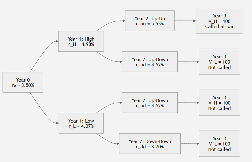
Binomial and Trinomial Lattices: These models discretize time (typically in six-month or one-year steps) to map out potential future interest rate pathways.
Arbitrage-Free Calibration: The interest rate lattice is mathematically calibrated so that the tree’s model-derived prices for option-free benchmark bonds match actual market prices exactly, ensuring the model remains “fair” and consistent with the spot curve.
Backward Induction (Recursive Valuation): Starting at the bond’s maturity (where cash flows are certain), analysts work backward from right to left. At each individual node, the present value of future cash flows is calculated by discounting at that node’s rate. If an option is eligible for exercise, the node’s calculated value is adjusted to the option’s exercise boundary (e.g., replaced by the call price if the calculated value exceeds it).
Option-Adjusted Spread (OAS): The constant spread added to all interest rates in the lattice to align the model’s theoretical price with the security’s actual market price. By explicitly modeling and adjusting for the cash-flow impact of the embedded option at every node, the OAS removes the option’s effect, leaving a pure credit and liquidity spread relative to the benchmark curve.

The Boundary of Lattices: Path-Dependence

Backward induction on a lattice requires interest-rate-path independence. For path-dependent structured securities (such as Mortgage-Backed Securities, where prepayment behavior depends heavily on historical interest-rate burnout), lattices fail because a node has no memory of how interest rates arrived there. In these instances, practitioners must deploy Monte Carlo simulation models to randomly project thousands of interest rate paths, calculate pathwise cash flows, and average their present values.

Callable and Putable Bonds

1. The Decomposed Anatomy of Bonds with Embedded Options

In fixed-income mathematics, embedded options are contingency provisions written directly into a bond’s indenture or offering circular. These options are fundamentally non-detachable; they cannot be separated from the underlying debt instrument or traded independently.

To value and analyze these hybrid instruments, financial theory decomposes them into their constituent parts:

Callable Bonds: A callable bond grants the issuer the right to redeem all or part of the debt prior to maturity, typically to refinance at lower rates if market yields fall or the issuer’s credit quality improves. Economically, the investor is long a straight bond and has sold (shorted) a call option to the issuer:

Value of Callable Bond=Value of Straight Bond − Value of Issuer Call Option

Because this option benefits the issuer and exposes the investor to reinvestment risk, callable bonds must sell at lower prices and offer higher yields than equivalent option-free straight bonds to entice buyers. Exercise styles are typically American (continuously callable), European (callable once on a specific date), or Bermudan (callable on specified dates, such as coupon anniversaries).

Putable Bonds: A putable bond grants the bondholder the right to sell the bond back to the issuer (usually at par value) on specified dates, typically when interest rates rise so they can reinvest the proceeds into higher-yielding securities. Economically, the investor is long both the straight bond and a put option:

Value of Putable Bond=Value of Straight Bond + Value of Investor Put Option

Because this option protects the investor, putable bonds sell at higher prices and lower yields than equivalent option-free bonds. Like callables, they are structured under American, European, or Bermudan rules, and can be structured as one-time put bonds or multiple put bonds.

2. Yield Curve Dynamics: Capping and Flooring Performance

The presence of embedded options alters how bonds respond to changes in the level and shape of the yield curve, establishing asymmetric boundaries:

Price Compression in Callable Bonds: When interest rates are high relative to the coupon rate, the call option is out of the money and highly unlikely to be exercised. Under this regime, the callable bond trades virtually in lockstep with a straight bond. However, as interest rates fall, the likelihood of an early call increases. The price of the callable bond departs from the straight bond and begins to compress near the call price (creating negative convexity), limiting the investor’s price appreciation.
The Yield Curve Shape Effect: The value of an embedded call option increases as the yield curve flattens or inverts. When the curve flattens or inverts, the forward rates on the lattice become lower, which materially increases the probability that interest rates will drop into the range where refinancing becomes highly economical for the issuer.
Downside Protection in Putable Bonds: Conversely, as interest rates rise, the price of a straight bond falls. For a putable bond, however, the ability to put the bond at par limits the price depreciation, acting as a natural hedge. If interest rates are very low, the put option is out of the money and the bond behaves exactly like a straight bond.

3. Valuation Under Volatility: Lattices and Backward Induction

To value callable and putable bonds in the presence of interest rate volatility, practitioners map out short-rate pathways using discrete binomial or trinomial lattices. The lattice must be mathematically calibrated so that its model-derived prices for option-free benchmark bonds match actual market prices exactly, ensuring the tree is “arbitrage-free”.

Once the calibrated tree is established, the arbitrage-free value is calculated by working from right to left using backward induction:

At each maturity node (Year 3), the terminal payoff is known with certainty (par plus the final coupon).
To step backward to the previous node (Year 2), the expected cash flows of the up and down states are averaged and discounted using that node’s forward rate (r∗):

For a callable bond, the value at any node Vt is restricted to the lesser of the calculated holding value and the call price:

V_t = min[Call Price, PV(Future Cash Flows)]

If the calculated value exceeds the call price, it is struck out and replaced by the call price, as the issuer would rationally choose to call the bond.

For a putable bond, the value at any node is adjusted to the greater of the calculated holding value and the put price:

V_t=max[Put Price, PV(Future Cash Flows)]

If the calculated value falls below the put price, the investor exercises the put, and the value is replaced by the put price.

The Volatility Trade-Off: Because the value of all options rises with expected interest rate volatility, higher volatility increases the call option’s value, which decreases the price of the callable bond. For a putable bond, higher volatility increases the put option’s value, which increases the price of the putable bond.

4. The Option-Adjusted Spread (OAS)

For risky bonds, rather than adjusting the cash flows themselves for credit defaults, the market convention is to add a constant spread to the rates in the binomial tree.

Definition: The Option-Adjusted Spread (OAS) is the constant basis-point spread that, when added to all of the forward rates in the binomial lattice, equates the model’s theoretical price to the observed market price of the option-embedded security.
Option Extraction: By modeling the option exercise explicitly at each node and adjusting the cash flows accordingly, the OAS successfully peels away the effect of the embedded option. The resulting spread is left to reflect only pure credit risk, liquidity premiums, and sector mispricings relative to the benchmark curve.
Volatility Sensitivity: For a given market price, if you assume a higher interest rate volatility in your model, the calculated value of the embedded call option rises. Because more of the total yield spread is now explained by the option’s value, the OAS of a callable bond decreases as volatility assumptions rise. Conversely, the calculated OAS of a putable bond increases under higher volatility assumptions.

5. Re-Engineering Risk Metrics: Curve Sensitivity & Convexity

Because interest rate changes alter a bond’s future expected cash flows, traditional yield-based metrics—such as modified duration or Macaulay duration—are mathematically invalid for bonds with embedded options. They assume cash flows remain static, which leads to severe underestimations of price risk. To accurately analyze option-embedded bonds, curve-based risk metrics are required:

A. Effective Duration

Effective (or option-adjusted) duration measures a bond’s sensitivity to a parallel shift in the benchmark yield curve (such as the sovereign par curve) rather than a shift in its own yield to maturity:

The inputs are generated by shifting the benchmark curve up and down by a small increment (ΔCurve), constructing the corresponding new interest rate trees, and calculating PV+ and PV− using the original constant OAS.

The effective duration of both callable and putable bonds is strictly capped by, and cannot exceed, the duration of an otherwise identical option-free straight bond.

Callable Bonds: When rates are high, effective duration is close to straight duration. As rates fall and the call option moves near or into the money, the effective duration shortens dramatically, eventually converging toward the duration of a straight bond maturing on the first call date.
Putable Bonds: When rates are low, effective duration is close to straight duration. As rates rise and the put option moves into the money, the effective duration shortens as the expected life of the security is reduced to the next put date.

B. One-Sided Durations

Because the price sensitivity of option-embedded bonds is highly asymmetrical near the exercise price (e.g., a callable bond is bounded on the upside but has unlimited downside), a standard two-sided effective duration can mask risk. Analysts calculate one-sided durations (an independent one-sided up-duration and a one-sided down-duration) to capture this asymmetry. For example, near-the-money callable bonds will exhibit a much larger one-sided up-duration than a down-duration, reflecting high vulnerability to rate increases but capped appreciation to rate declines.

C. Key Rate Durations (Partial Durations)

Key rate durations measure sensitivity to a yield curve shift at a specific maturity segment while holding other rates constant, allowing managers to identify shaping risk.

For high-coupon callable bonds (highly likely to be called), the key rate duration shifts entirely from the bond’s final maturity to the call date (e.g., a 30-year callable bond behaves strictly like a 10-year option-free bond, showing zero sensitivity to 30-year rate shifts and high sensitivity to the 10-year rate).
For low-coupon putable bonds (highly likely to be put), the key rate duration similarly shifts from the maturity date and concentrates around the 10-year put date.

D. Effective Convexity

Effective convexity measures how a bond’s effective duration changes as interest rates shift:

Callable Bonds: Exhibit negative effective convexity (concavity) when interest rates are low and the call option moves near or into the money. This reflects the fact that as rates fall, the potential price appreciation is compressed, making the price-yield curve concave.
Putable Bonds: Always maintain positive effective convexity. As rates rise, the downside is floored at the put price, meaning the price-yield curve remains highly convex.

Convertible Bonds

In the broader context of fixed-income analysis, embedded options represent contingency provisions written directly into a bond’s indenture that grant either the issuer or the bondholder the right (but not the obligation) to alter the scheduled cash flows . Because these options are legally attached to the security, they cannot be detached or traded independently from the underlying debt—known as the straight bond .

Among the various types of option-embedded debt, convertible bonds represent a highly unique, hybrid class of securities that bridge the gap between fixed income and equity .

1. The Anatomy of a Convertible Bond

A convertible bond consists of a package combining a straight, option-free bond and an embedded equity call option on the issuer’s common stock . This option grants the bondholder the right to exchange the bond for a specified number of common shares during a predetermined conversion period at a set conversion price .

Because this equity option is highly valuable to investors, convertible bonds trade at higher prices and offer significantly lower yields than otherwise identical non-convertible straight bonds . This below-market coupon rate reduces interest expenses for the issuing company .

2. Decomposing and Valuing Convertible Bonds

Under the arbitrage-free framework, the value of a convertible bond is modeled by decomposing the security into its constituent components . The baseline valuation of a plain-vanilla convertible bond is expressed as:

Value of Convertible Bond = Value of Straight Bond + Value of Equity Call Option on the Issuer’s Stock

However, issuers frequently combine multiple embedded options within a single structure . Most notably, convertible bonds are often callable by the issuer (to force conversion or refinance if interest rates fall) and may also be putable by the investor (to protect against rising interest rates or credit downgrades) . Under the arbitrage-free lattice framework, these complex interactions are valued recursively as follows :

Callable Convertible Bond:

Value = Value of Straight Bond + Value of Equity Call Option − Value of Issuer Call Option

Callable Putable Convertible Bond:

Value = Value of Straight Bond + Value of Equity Call Option − Value of Issuer Call Option + Value of Investor Put Option

3. Key Analytical Metrics and the “Moving Floor”

To evaluate the relative value of a convertible bond, analysts monitor several standard metrics:

Conversion Ratio: The number of common shares received per bond upon conversion . It is equal to the bond’s par value divided by its initial conversion price.
Conversion Value (Parity Value): The equity-equivalent value of the bond if converted immediately at current market levels.

Conversion Value = Underlying Share Price × Conversion Ratio

Minimum Value (The Floor): A convertible bond cannot trade below its minimum value without triggering immediate risk-free arbitrage . This floor is established as:

Minimum Value = max(Conversion Value, Straight Bond Value)

Crucially, the straight bond value acts as a “moving floor.” It is not static; it fluctuates continuously in response to changes in benchmark interest rates and issuer-specific credit spreads .

Market Conversion Price: The effective stock price paid by an investor purchasing the bond in the secondary market .

Market Conversion Premium: The extra amount paid per share by purchasing the convertible bond rather than buying the stock directly . This premium is paid because the bond offers downside protection (via the straight bond floor) that direct equity ownership lacks .

4. The Three Risk-Return Regimes (Trading Profiles)

Depending on where the issuer’s stock price trades relative to the conversion price, a convertible bond behaves according to three distinct risk-return regimes :

The Convertible Hybrid Spectrum

Feature	Busted / Bond Equivalent	Hybrid Regime	Stock Equivalent
Stock price vs. conversion strike	Far below strike	Near strike	Far above strike
Conversion option status	Out of the money	Near the money	Deep in the money
Primary price driver	Interest rates and credit spreads	Both bond and equity factors	Underlying stock price
Downside behavior	Supported by the straight-bond floor	Downside is bounded by the bond floor	Primarily exposed to stock-price declines
Upside behavior	Limited equity participation	Meaningful upside participation	Moves approximately dollar-for-dollar with the stock
Interest-rate sensitivity	High	Moderate	Low
Overall character	Bond-like	Bond–equity hybrid	Equity-like

Spectrum: Bond-like ⟶ Hybrid ⟶ Equity-like

Bond Equivalent (Busted Convertible): When the underlying stock price is well below the conversion price, the equity option is deep out of the money and virtually worthless . The security trades strictly on its fixed-income characteristics, meaning its price is driven by interest rate movements, credit spreads, and the straight bond floor .

Stock Equivalent: When the underlying stock price is well above the conversion price, the call option is deep in the money . The bond trades in lockstep with the share price (following the conversion value) and becomes virtually insensitive to interest rate fluctuations .
The Hybrid Regime: When the stock price is close to the conversion price, the bond exhibits highly desirable asymmetric behavior . On the upside, as the stock price increases, the bond price rises and begins to participate in the equity gains . On the downside, if the stock price falls, the bond’s price depreciation is cushioned and eventually floored by the straight bond value .

5. Special Optionalities: Forced Conversion, Warrants, and CoCos

Forced Conversion: In callable convertible bonds, if the stock price rises significantly above the conversion price, the issuer has an incentive to call the bond . This forces the bondholders to convert their debt into shares (as the conversion value exceeds the call price), allowing the issuer to wipe out its debt, extinguish coupon liabilities, and permanently recapitalize its balance sheet .
Warrants: While similar to conversion options, warrants are “attached” options rather than embedded options . A warrant is a separate, tradable security that can be detached and traded independently of the underlying bond, acting as a yield-enhancing “sweetener” at issuance .
Contingent Convertible Bonds (CoCos): Primarily issued by European financial institutions, CoCos differ fundamentally from traditional convertibles because they convert on the downside . If a bank’s capital ratio falls below a regulatory minimum, the bonds automatically write down or convert into equity to recapitalize the bank and prevent systemic collapse . Because this conversion is automatic and forces losses on investors, CoCos must offer a much higher yield than traditional convertible bonds .

Contingent Convertible (CoCos)

1. Conceptual Framework of CoCos as Embedded Options

In fixed-income mathematics, an embedded option represents a contingency provision written into a bond’s indenture that grants either the issuer or the bondholder a specific right—but not the contractual obligation—to alter the bond’s schedule of cash flows.

Contingent convertible bonds (popularly nicknamed “CoCos”) represent a highly specialized class of hybrid debt carrying a unique embedded option: a contingent write-down or automatic conversion provision. CoCos differ fundamentally from traditional option-embedded securities because they do not grant discretionary exercise rights to either the investor or the issuer; instead, the embedded option is triggered automatically by a pre-defined external event.

2. Downside Conversion: CoCos versus Traditional Convertibles

Traditional convertible bonds are designed to protect investors on the downside while allowing them to participate in the issuer’s equity growth. The embedded call option in a traditional convertible operates as follows:

Discretion: Conversion is executed at the sole option of the bondholder.
Upside Direction: Conversion is designed to occur on the upside—specifically when the issuing company’s share price increases above the conversion price, making equity exchange highly profitable.

In contrast, CoCos are structured to convert on the downside to protect the issuer’s solvency rather than the investor’s returns:

Automation: Conversion is entirely automatic and non-discretionary once the trigger event occurs.
Downside Direction: The embedded option is activated when the issuer experiences severe financial distress, forcing bondholders to absorb losses on the downside.

3. The Trigger Mechanic and Issuing Motivations

The automatic activation of a CoCo’s downside option is dictated by a specific regulatory trigger. For banking institutions, this trigger is typically tied to capital preservation:

The Trigger Event: The option automatically activates if the bank’s core capital—such as its core Tier 1 capital ratio—falls below the minimum threshold mandated by financial regulators.
The Downside Action: Upon hitting this trigger, the CoCo immediately and automatically converts into common stock or undergoes a principal write-down.
Systemic Risk Mitigation: This automatic exercise immediately recapitalizes the bank and lightens its debt burden without forcing it into formal bankruptcy, dramatically reducing its risk of default and lowering market-wide systemic risk. Consequently, these instruments are primarily issued by European financial institutions to establish a robust regulatory capital cushion.

4. Risk-Return Profile and the Pricing Premium

Because the embedded option in a CoCo automatically forces losses onto the investor on the downside (by converting debt into depreciating equity or wiping out principal), it represents an exceptionally high-risk investment. Furthermore, CoCos are typically deeply subordinated in the issuer’s capital structure.

To entice risk-averse investors to accept this downside optionality and subordination, issuers must compensate them ex-ante. Thus, CoCos must offer a significantly higher yield (or a higher coupon rate) than traditional convertible bonds or otherwise identical non-convertible debt.

5. Advanced Hybridization: “CoCoCos”

The financial markets have also developed a further option-embedded variation known as Convertible Contingent Convertible bonds (“CoCoCos”). A CoCoCo combines the upside opportunity of a traditional convertible with the downside protection of a CoCo within a single security:

On the Upside: The investor retains a traditional, discretionary call option to convert the debt into equity if the common stock price appreciates.
On the Downside: The bond remains subject to automatic, mandatory conversion or principal write-down if the bank’s regulatory capital ratios are breached.

Other Instruments

Traditional fixed-income analysis is historically anchored in option-free, fixed-rate straight bonds . However, modern global debt capital markets feature a vast array of alternative, customized, and structured instruments designed to solve specific asset-liability matching problems, manage unique risks, or target specific investor segments .

The sources categorize and analyze these “other instruments” across several distinct functional and credit families:

1. Money Market and Liquidity Instruments

For short-term cash management and funding, banks, corporations, and institutional investors rely on a specialized suite of money market instruments that typically mature in one year or less :

Commercial Paper (CP): These are unsecured, short-term promissory notes representing a debt obligation of the issuer . In the U.S. market, to avoid the time and expense of SEC registration, CP maturities are strictly capped below 270 days and are typically issued on a discount basis . Conversely, Eurocommercial paper (ECP) can mature up to 364 days and is typically quoted on an interest-bearing (add-on rate) basis .
Medium-Term Notes (MTNs): Despite their name, MTNs are not defined by intermediate maturities; instead, they are characterized by being offered continuously to investors through an agent, giving issuers maximum funding flexibility . MTNs can be structured with customized features and can span maturities from short-term floaters to 100-year “century bonds” .
Repurchase Agreements (Repos): Structurally equivalent to a collateralized loan, a repo involves the sale of a security (the collateral) with a simultaneous agreement by the seller (the borrower of cash) to buy it back at a higher price (reflecting the repo rate) in the future .
Negotiable Certificates of Deposit (CDs): Large-denomination bank deposits with specified maturities and interest rates that can be actively traded in the secondary market prior to maturity .

2. Complex Floating-Rate and Structured Coupon Formats

To manage interest rate risk or cash-flow constraints, issuers utilize coupon structures that deviate from standard flat, fixed rates :

Inverse Floaters: Unlike a traditional Floating-Rate Note (FRN) whose coupon moves positively with a reference rate , an inverse floater’s coupon rate rises when interest rates fall . It is valued residually: Collateral Value = Floater Value + Inverse Floater Value . It functions as a highly leveraged long position funded with borrowed short-term funds , resulting in an interest rate risk (duration) that is a multiple of the underlying collateral’s duration .
Range Notes (Range Floaters): Structured floaters where coupon payments are contingent on the number of days a reference rate (like Libor) remains within a pre-established collar or band . If the rate moves outside the band, the coupon for that day drops to zero .
Payment-in-Kind (PIK) & PIK Toggle Notes: PIK bonds allow the issuer to pay periodic interest in the form of additional bonds or common stock rather than cash . PIK toggle notes give the borrower the discretion to switch between cash and in-kind payments based on earnings or cash-flow triggers, which is highly useful in leveraged buyout (LBO) structures .
Step-Up Callable Notes: These bonds feature a pre-set coupon schedule that increases (steps up) at specified intervals . Because they are typically callable, the step-up feature provides investors with a partial hedge against rising interest rates, while the call option allows the issuer to refinance if rates decline .

3. Inflation-Linked, Index-Linked, and Hybrid Notes

To insulate portfolios from macroeconomic volatility, financial engineers link bond payments directly to price or asset indices :

Inflation-Linked Bonds (Linkers): These protect investors from purchasing-power erosion by linking a bond’s coupon and/or principal payments to a consumer price index . The most common structure is the Capital-Indexed Bond (such as US TIPS), where the principal is adjusted for inflation over time while a fixed real coupon rate is applied to the adjusted principal . Other variations include Interest-Indexed Bonds (adjusting interest payments only) and Zero-Coupon-Indexed Bonds (adjusting only the principal paid at maturity) .
Equity-Linked Notes (ELNs): Hybrid, principal-protected instruments where the final payment is tied to the return of a stock market index . An ELN mathematically behaves like a zero-coupon bond combined with an equity call option .
Currency Option and Dual-Currency Bonds: Dual-currency bonds pay periodic coupon interest in one currency and the principal par value at maturity in another currency . Currency option bonds grant bondholders the right to choose which of two currencies they want to receive for each individual interest and principal payment .

4. Credit Derivatives and Risk Transfer Instruments

The financial markets have decoupled credit default risk from physical bond ownership, leading to a massive expansion of structured credit instruments :

Credit Default Swaps (CDS): Standardized over-the-counter contracts where a protection buyer pays a periodic premium to a protection seller in exchange for a payout if a reference entity defaults .
- The CDS-Bond Basis: This compares credit spreads in the cash bond market with the CDS market . A critical distinction is that physical bond positions levered in the repo market are subject to financing risk (the risk that short-term repo funding dries up or overnight rates rise), whereas CDS positions bypass this risk due to implicit financing built into the contract to maturity .
Credit Risk Transfer (CRT) Securities: Issued by housing agencies (like Fannie Mae’s CAS), CRTs are debt securities that transfer the credit default risk of a reference pool of residential mortgages to private investors . The tranches are structured in a hierarchical waterfall where actual investor principal is written down sequentially as defaults in the reference pool occur .
Covered Bonds: Primarily issued by European financial institutions, covered bonds are debt obligations backed by a segregated, dynamic pool of high-quality mortgage or public-sector loans (the “cover pool”) . Unlike securitized products (ABS/MBS) where the assets are sold to a separate Special Purpose Vehicle , covered bonds remain on the issuer’s balance sheet, providing investors with dual recourse to both the general assets of the bank and the collateral pool .

Floating-Rate Notes (FRN)

Core Mechanics and Pricing of Floating-Rate Notes

Floating-Rate Notes (FRNs, or floaters) are debt securities with coupon interest rates that vary dynamically over the security’s life. They are issued across all sectors of the bond market—including government, corporate, municipal, and structured finance—and typically pay interest quarterly.

The periodic coupon rate of a standard, option-free floater is determined by a simple formula:

Coupon Rate = Reference Rate ± Quoted Margin

The quoted margin (or spread) is a constant adjustment in basis points established at issuance to reflect the credit risk of the issuer relative to the benchmark index. The reference rate is a short-term money market interest rate (such as Libor, Euribor, Hibor, Sibor, or the Secured Overnight Financing Rate [SOFR]) that resets at designated intervals.

Because their coupons adjust to match prevailing interest rates on each reset date, floaters are highly defensive securities that experience very little interest rate risk compared to fixed-rate bonds. If there is no change in the issuer’s credit risk, an FRN’s flat price will stay close to par on coupon reset dates. However, if the market’s required margin (or discount margin) changes—typically due to fluctuations in the issuer’s credit quality or market liquidity—the flat price will deviate from par. An increase in credit risk drives the required margin above the quoted margin, forcing the floater to trade at a discount. Conversely, if credit quality improves, the required margin drops below the quoted margin, and the floater trades at a premium. To evaluate these dynamics, practitioners utilize spread measures such as the spread for life (simple margin), adjusted simple margin, adjusted total margin, and the discount margin.

Quantifying Floater Sensitivity: Index vs. Spread Duration

Because floaters are exposed to two distinct risk components (interest rates and credit spreads), analysts divide their price sensitivity into two separate measures:

Index Duration: This measures the floater’s price sensitivity to changes in the reference rate while holding the quoted margin constant. The interest rate duration of a floater is extremely small, as it is bounded by the time remaining to the next coupon reset date (e.g., a semi-annual reset floater has a duration of less than six months).
Spread Duration: This measures the sensitivity of the floater’s price to changes in the quoted margin or market credit spread, assuming the reference rate remains unchanged.

Embedded Options: Caps, Floors, and Collars

Many floating-rate securities incorporate embedded options that restrict the coupon’s ability to float, creating asymmetrical risk profiles that must be valued using binomial interest rate lattices:

Capped Floaters: An embedded cap sets a maximum limit on the coupon rate paid by the issuer. This issuer-contingent option protects the borrower from rising rates but detriments the investor. If interest rates rise above the cap, the coupon rate becomes fixed, and the floater begins to trade at a discount and assume the duration risk of a standard fixed-rate bond. Its value is modeled as:

Value of Capped Floater=Value of Straight Bond−Value of Embedded Cap

Floored Floaters: An embedded floor sets a minimum coupon rate, protecting investors against falling interest rates. Because this option benefits the bondholder, it increases the bond’s value:

Value of Floored Floater=Value of Straight Bond+Value of Embedded Floor

Collared Floaters: A collared floater incorporates both a cap and a floor, restricting the coupon rate to a pre-specified band.

FRNs in the Broader Context of “Other Instruments”

To understand how FRNs fit into the larger fixed-income cosmos, they must be analyzed alongside other complex, synthetic, and derivative instruments:

A. Inverse Floaters

Unlike ordinary floaters, the coupon of an inverse floater moves in the opposite direction of the reference rate. They are typically engineered by investment banks by splitting a fixed-rate bond (collateral) into a standard capped floater and an inverse floater. The general coupon formula is:

Coupon Rate=Fixed Rate − (Leverage × Reference Rate)

The leverage represents the ratio of the par value of the floater to the inverse floater. Economically, owning an inverse floater is equivalent to buying the fixed-rate collateral and shorting (selling) the capped floater. Because shorting a floater is equivalent to borrowing funds at the floating rate, this position represents a highly leveraged long position in the collateral. Consequently, assuming the floater’s duration is close to zero, the price sensitivity of the inverse floater is highly magnified:

Duration of Inverse Floater = (1 +Leverage) × Duration of Collateral

B. Interest Rate Swaps (IRS)

There is a direct mathematical connection between floaters and interest rate swaps. An interest rate swap can be interpreted as a package of long and short cash market instruments. For instance:

A fixed-rate receiver (floating-rate payer) is equivalent to a long position in a fixed-rate bond and a short position in a floating-rate bond.
A fixed-rate payer (floating-rate receiver) is equivalent to a long position in a floating-rate bond financed by borrowing on a fixed-rate basis (shorting a fixed-rate bond).

The interest rate sensitivity of a swap is modeled using this bond equivalence. The dollar duration of a swap equals the difference between the dollar duration of the fixed-rate bond and the floating-rate bond. Because the duration of the floating-rate bond is so small (less than the time to the next reset date), most of the interest rate sensitivity of a swap is driven entirely by the duration of the fixed-rate bond.

C. Range Notes

A range note (or range floater) is a structured floater where the coupon is contingent upon daily interest rate dynamics. It pays the reference rate only for the days that the rate remains within a pre-established collar or band; if the rate moves outside the band, the coupon for that day falls to zero.

D. US Treasury Floating-Rate Notes

Historically, the largest sovereign issuers did not issue floaters, but in January 2014, the US Treasury introduced two-year FRNs. These sovereign floaters pay a variable rate tied to the weekly 13-week T-bill auction rate plus a fixed spread. This design locks in two-year funding for the government at short-term bill rates, while offering yield-seeking investors a safe, slightly higher-spread alternative to rolling over short-term T-bills.

Inverse Floaters

Core Mechanics and Structure of Inverse Floaters

An inverse floating-rate security (or inverse floater) is a specialized debt instrument whose coupon rate moves in the opposite direction of a designated short-term reference rate (such as Libor or Euribor). When the reference interest rate increases, the coupon rate on the inverse floater declines; conversely, when the reference rate decreases, the inverse floater’s coupon rate rises. Because of this pricing dynamic, inverse floaters are typically favored by investors who anticipate a decline in interest rates.

An investment banker or dealer typically creates an inverse floater synthetically by splitting a fixed-rate bond (known as the collateral) into two separate parts: a floating-rate note and an inverse floater.

The Leverage Multiplier: The general coupon formula for an inverse floater is expressed as:

Coupon Rate = Fixed Rate − (Leverage × Reference Rate)

Here, leverage (or coupon leverage) is the ratio of the par value of the companion floater to the par value of the inverse floater. For example, if $400 million of collateral is split into a $300 million floater and a $100 million inverse floater, the leverage is 3 ($300M/$100M).

The Cap and Floor Constraint: The combined interest paid to the floater and the inverse floater cannot exceed the total coupon interest generated by the underlying collateral. Because a dramatic rise in the reference rate could theoretically drive the inverse floater’s coupon below zero, a floor (typically set at zero) is placed on the inverse floater’s coupon rate. To maintain the collateral’s cash flow balance, the companion floater must consequently have a maximum interest rate limit, turning it into a capped floater.

Valuation and the “Levered Long” Interpretation

Because future reference rates are uncertain, valuing an inverse floater directly from its cash flows can be complex. However, arbitrage-free pricing dictates that the sum of the components must equal the value of the underlying collateral:

Collateral Value = Capped Floater Value + Inverse Floater Value

Therefore, the value of an inverse floater is derived residually:

Inverse Floater Value = Collateral Value − Capped Floater Value

This valuation relationship yields a critical economic interpretation of the investor’s position:

Long an Inverse Floater = Long a Fixed – Rate Collateral+ Short a Capped Floater

Because shorting a floater is mathematically equivalent to borrowing funds at an uncertain floating rate, the owner of an inverse floater has effectively purchased a fixed-rate bond using borrowed funds. This makes an inverse floater a highly levered long position in the underlying fixed-rate collateral.

Magnified Interest Rate Risk (Duration)

Because valuations are additive, the durations of the components (when properly weighted) must also sum to the duration of the collateral. Under the standard assumption that the companion floater resets frequently and thus has an interest rate duration close to zero, the entire interest rate risk of the collateral is concentrated on the inverse floater.

The price sensitivity of the inverse floater is determined by multiplying the collateral’s duration by the leverage of the structure:

Duration of an Inverse Floater = (1 + Leverage) × Duration of Collateral

For example, if the collateral has a duration of 7 and the leverage of the split is 3, the inverse floater will have an effective duration of 28. This explains how a fixed-income instrument can possess a duration significantly greater than the actual maturity of its underlying collateral.

Connection to Other Instruments: Interest Rate Swaps

In the larger context of debt derivatives, inverse floaters share strong structural and risk characteristics with interest rate swaps.

An interest rate swap is an OTC contract where counterparties exchange periodic fixed-rate and floating-rate interest payments. In this framework:

A floating-rate payer (fixed-rate receiver) in a swap holds a synthetic cash-market position equivalent to being long a fixed-rate bond and short a floating-rate bond.
With the exception of the protective cap embedded in the companion floater, the cash flow profile of an inverse floater is virtually identical to this swap position, as the investor receives a fixed return and pays a variable floating-rate interest expense.

Inflation-Linked Bonds (Linkers)

The Core Premise and Mechanics of Inflation-Linked Bonds

Standard fixed-income instruments expose investors to inflation risk because their contractual nominal cash flows are fixed. If a country experiences inflation, the purchasing power of these fixed payments is systematically eroded. To mitigate this risk, national governments and corporate issuers utilize inflation-linked bonds (popularly called “linkers”), which are structured to adjust coupon payments, principal repayments, or both, in line with a consumer price index.

While nominal coupon bonds provide a fixed dollar or nominal return, linkers offer investors a fixed real rate of return that is insulated from purchasing power risk. The real rate of return is approximately equal to the nominal interest rate minus the rate of inflation.

Structural Designs of Inflation Indexing

The cash flows of index-linked bonds are structured and adjusted using several distinct methods:

Capital-Indexed Bonds: This represents the most common structured linker format. The bond pays a fixed real coupon rate, but this rate is applied to a principal amount that increases or decreases in line with inflation. Consequently, both the periodic coupon payments and the principal repayment at maturity are adjusted. Examples include US TIPS (Treasury Inflation-Protected Securities), which pay interest twice a year and are tied to the US Consumer Price Index (CPI-U). TIPS also feature deflation protection: if a period of deflation occurs, the principal may decrease, but at maturity, the investor is paid the greater of the original par value or the inflation-adjusted principal. Other countries issuing capital-indexed bonds include Australia, Canada, New Zealand, and the United Kingdom.
Zero-Coupon-Indexed Bonds: These pay no periodic coupon interest. Instead, the inflation adjustment is applied strictly to the principal amount paid at maturity. This structure has been issued by the government of Sweden.
Interest-Indexed Bonds: These maintain a fixed nominal principal amount at maturity, but the periodic coupon payments are adjusted for inflation. This structure was briefly issued by the Australian government in the late 1980s but did not become a dominant market format.
Indexed-Annuity Bonds: These are fully amortized bonds rather than bullet bonds. The regular annuity payment (which combines both interest and principal repayment) increases in line with inflation. Local governments in Australia have historically issued these instruments.

Global Issuers and Motivations

While national governments are the primary issuers of linkers, corporate issuers—including both financial and non-financial companies—increasingly utilize them. Globally, sovereign issuers of linkers generally fall into three functional categories:

Macroeconomic Necessity: Countries such as Brazil, Chile, and Colombia issued inflation-linked bonds because they experienced extremely high inflation and offering linkers was their only viable method to raise funds from wary capital markets.
Credibility and Demand: The United Kingdom (which issued its first Retail Price Index-linked gilt in 1981), Australia, and Sweden issued linkers to demonstrate their commitment to disinflationary policies and to satisfy investor demand for inflation hedges.
Social Welfare: Nations like the United States (which introduced TIPS in 1997), Canada, Germany, and France issue linkers primarily to provide long-term assets that offer risk-free real returns.

To track inflation, different countries tie their securities to localized benchmarks, such as the Consumer Price Index (CPI-U) in the United States, the Retail Price Index (RPI) in the United Kingdom, and either the French CPI (excluding tobacco) or the Eurozone’s Harmonized Index of Consumer Prices (HICP) in France.

Context Within Alternative and “Other” Instruments

In the broader context of debt capital markets, linkers play a unique dual role as both protective vehicles and crucial macroeconomic benchmark tools:

Measuring Inflation Expectations: By comparing the yield of a nominal government bond with the yield of an otherwise identical linker (such as TIPS), investors can directly extract the breakeven inflation rate. The spread between these yields represents the market’s expected inflation rate plus the premium required to bear inflation risk.
Imperfections in Indexing: While linkers are highly defensive relative to traditional fixed-rate straight bonds, they do not completely eliminate inflation risk. This is because the underlying consumer price index used by the contract may be an imperfect proxy for the actual inflation experienced by a specific investor.
Contrasting with Other Options: Unlike standalone or embedded interest rate options (such as caps or floors on floaters, which alter coupon cash flows based on short-term interest rates), the automatic scaling in linkers is tied strictly to a macroeconomic index. Additionally, while credit-linked coupon bonds alter cash flows based on microeconomic issuer risk (rating changes), linkers isolate macro-level purchasing power shifts, which is why they are often grouped under “index-linked” or hybrid strategies alongside equity-linked notes (ELNs).

Payment-in-Kind (PIK) Bonds

Payment-in-Kind (PIK) bonds represent a highly specialized category of corporate debt securities characterized by their flexible coupon payment structures . Rather than requiring the issuer to pay periodic interest exclusively in cash, a PIK bond typically allows the interest obligation to be satisfied through the issuance of additional amounts of the bond itself (additional debt) or through common shares .

Issuer Motivations and Credit Risk

PIK structures are primarily utilized by corporate borrowers facing significant capital constraints or anticipated cash flow pressures . By preserving cash that would otherwise be earmarked for immediate interest payments, the issuer gains crucial financial flexibility to manage its operations or service other obligations .

Consequently, these instruments are widely deployed to finance companies carrying exceptionally high debt burdens, particularly those undergoing a leveraged buyout (LBO) . Because deferring cash interest payments naturally elevates the credit risk borne by the lender, investors recognize this heightened exposure and systematically demand a higher yield to hold PIK coupon bonds compared to standard cash-pay debt .

Key PIK Variations and the Toggle Mechanism

The sources outline several distinct structures under the broader PIK umbrella:

Common Stock Settlement: In some PIK arrangements, the issuer pays the coupon by distributing common shares of equivalent value to the bondholders rather than issuing more debt .
PIK Toggle Notes: This variation grants the borrower the optionality, on an interest-period-by-interest-period basis, to decide whether to pay interest in cash, in kind (additional bonds), or via a designated mix of both .
Indenture Triggers: While the choice of payment method in a toggle note is frequently left to the borrower’s sole discretion, the bond indenture can also tie this payment decision directly to objective corporate performance metrics, such as specific earnings or cash flow triggers .

The Larger Context of Alternative Coupon Structures

Within the broader spectrum of fixed-income instruments, PIK bonds are part of a family of non-vanilla coupon payment structures engineered to bridge different credit and financing needs:

Deferred Coupon Bonds: Like PIKs, these bonds offer cash-preservation benefits to the issuer by paying no coupon in the early years of the bond’s life, followed by higher interest payments in the remaining years .
Zero-Coupon Bonds: These represent the extreme of interest deferral, paying no periodic coupon whatsoever and instead trading at a deep discount to par value before redeeming at par at maturity .
Credit-Linked Coupon Bonds: Unlike PIK bonds, which accommodate cash flow strains by changing the form of payment, credit-linked bonds adjust the interest rate itself, raising or lowering the coupon rate dynamically in response to changes in the issuer’s credit rating .

Derivatives and Funding

In the broader landscape of fixed-income analytics, the worlds of derivatives and funding are deeply and mathematically intertwined. While physical bonds require direct capital outlays or explicit cash-market borrowing, derivatives are frequently used to synthetically replicate these exact exposures, fundamentally altering how financial institutions manage leverage, liquidity, and balance sheet risk.

1. Repurchase Agreements (Repos) as the Operational Engine of Funding

At the core of fixed-income funding is the repurchase agreement (repo) market, which is structurally a legal sale and repurchase of a security but functions economically as a secured, collateralized loan .

The Mechanics of Collateralized Financing: A borrower of cash (the repo seller) delivers securities to the lender (the repo buyer) as collateral, agreeing to buy them back at a higher price (reflecting the negotiated repo rate) in the future .
Risk Management and Margining: To insulate cash lenders from counterparty default and price volatility, repos employ a haircut (or initial margin)—reducing the loan amount below the market value of the collateral —and utilize daily variation margin calls to maintain that buffer as asset prices fluctuate . Furthermore, repo transactions enjoy a crucial legal safe harbor from standard bankruptcy stays, allowing lenders to immediately liquidate collateral in a default scenario .
Funding Strategies: Beyond basic cash management , dealers and investors utilize repos for long financing (using leverage to fund bond inventories or magnify investment returns) , short financing (using reverse repos to borrow specific “special” securities to cover short sales) , and collateral swaps (exchanging illiquid corporate bonds for liquid Treasuries) .

2. The Economic Equivalence of Derivatives and Leveraged Cash Positions

Many derivative structures are mathematically designed to replicate cash bond positions funded through the repo market:

A. Interest Rate Swaps (IRS) as Leveraged Funding

An interest rate swap can be interpreted as a package of cash flows that perfectly mimics buying a bond with borrowed funds .

A fixed-rate payer (floating-rate receiver) holds a synthetic position equivalent to being long a floating-rate bond and borrowing the cash to purchase it on a fixed-rate basis (effectively shorting a fixed-rate bond) .
Conversely, a fixed-rate receiver (floating-rate payer) holds a position equivalent to buying a fixed-rate bond and financing that purchase at a floating reference rate (like SOFR or Libor) . This allows institutions like pension funds to dramatically increase their interest rate sensitivity (duration) to match liabilities without deploying massive upfront cash .

B. Credit Default Swaps (CDS) vs. Cash Bond Financing (Financing Risk)

Selling CDS protection is economically analogous to buying a corporate bond and financing its purchase with a term repo matching the bond’s maturity . However, a massive operational divide exists between the two:

Because very long-term corporate repo markets do not exist, a cash market investor attempting to earn a credit spread via leverage must continuously roll over short-term or overnight repo . This exposes the investor to severe financing risk—the risk that short-term repo rates spike or that lenders refuse to roll the funding completely during a market panic, forcing a fire sale of the underlying bonds .
A CDS position embeds implicit financing to maturity directly within the derivative contract, insulating the protection seller from overnight repo rollover risks .

C. Leveraged Coupon Mimicry: Inverse Floaters

An inverse floater represents a highly levered long position in its underlying collateral bond . Synthetically, the owner of an inverse floater has purchased a fixed-rate bond and sold (shorted) a capped companion floater . Because shorting a floater is equivalent to borrowing funds at an uncertain floating rate, the investor has effectively established a levered long position in a fixed-rate bond using borrowed funds .

3. Systemic Funding Risks, Regulation, and Market Stress

Because leveraged fixed-income positions rely so heavily on short-term wholesale funding, they are highly sensitive to market-wide liquidity strains and regulatory constraints:

The Danger of Overnight Rolls: While rolling over overnight repo is cheap in calm markets, it is structurally unstable . During major market dislocations, prime brokers often reduce risk by raising haircuts or cutting credit lines, making it extremely difficult to fund even high-quality assets like Treasury securities .
The Impact of Bank Regulation: Modern post-crisis bank regulations, such as the Liquidity Coverage Ratio (LCR), the Net Stable Funding Ratio (NSFR), and the Supplementary Leverage Ratio (SLR), legally limit short-term wholesale funding and penalize banks for holding massive, low-yield repo assets on their balance sheets . This regulatory backdrop can prevent banks from acting as liquidity providers even when repo rates spike to highly profitable levels .
The Cautionary Case of MF Global: In 2011, MF Global engaged in massive repo-to-maturity (RTM) transactions, buying short-term sovereign debt and financing it with repo agreements that matured on the exact same dates . While designed to lock in net interest spreads and keep the leverage off-balance-sheet under the accounting rules of the time , the firm remained exposed to collateral margin calls . As sovereign credit spreads widened, clearinghouses and counterparties raised haircuts dramatically, triggering a liquidity squeeze that led to the firm’s collapse .

Interest Rate Swaps

Swaps as Synthetic Cash Instruments and Leveraged Positions

In modern fixed-income mathematics, interest rate swaps (IRS) are contracts where counterparties agree to exchange a sequence of interest payments based on a specified notional principal. From an analytical perspective, a swap position can be interpreted as a package of long and short cash market instruments:

Paying Fixed (Receiving Floating): Economically equivalent to a leveraged short position in a bond. The fixed-rate payer is synthetically long a floating-rate note (FRN) and short a fixed-rate bond (borrowing on a fixed-rate basis to finance the purchase of the floating asset).
Receiving Fixed (Paying Floating): Economically equivalent to a leveraged long position in a bond. The fixed-rate receiver is synthetically long a fixed-rate bond and short a floating-rate bond, replicating a scenario where an investor purchases a fixed-rate bond using funds borrowed at a variable, short-term rate.

Because of this replication, the dollar duration of a swap from the receiver’s perspective is simply the difference between the dollar durations of the underlying fixed-rate and floating-rate bonds. Since a floating-rate bond resets its coupon periodically, its duration is highly restricted (always less than the time to the next reset date). Consequently, nearly all of the interest rate sensitivity (duration risk) of a swap is driven entirely by its fixed-rate leg.

The Funding Engine: Applications across Financial Sectors

Because swaps represent leveraged positions that require no upfront principal exchange, they serve as powerful funding and balance-sheet-management tools:

1. Bank Asset-Liability Management (ALM)

Banks naturally fund themselves with short-term, floating-rate deposits, but borrowers often demand the security of long-term fixed-rate loans. To eliminate this mismatch, banks use back-to-back swaps: they extend a floating-rate loan, receive fixed from the borrower, and pay fixed to a swap dealer. This synthetically locks in a fixed rate for the borrower while maintaining a floating-rate asset on the bank’s balance sheet. Conversely, to secure stable, non-withdrawable funding, banks can issue long-term fixed-rate debt and enter an IRS to receive fixed and pay floating, synthetically creating long-term floating-rate debt.

2. Pension Liability Hedging

Defined-benefit pension plans carry exceptionally long-duration liabilities. Because long-maturity corporate bonds are scarce, pension managers often experience a duration gap. By receiving fixed on long-term swaps, pension funds can match the massive duration of their liabilities. Crucially, this derivative strategy requires no upfront capital (except for margin), allowing the fund to remain fully invested in active, return-generating corporate credits.

3. Pre-Hedging Corporate Debt Sales

Corporations planning future bond sales face the risk of rising interest rates in the interim. They can “pre-hedge” this risk by paying fixed today on a forward-starting swap. If market rates rise, the higher interest cost on the subsequent debt issuance is economically offset by the positive net present value (NPV) generated by the swap.

4. Sovereign Funding Optimization

During the Eurozone debt crisis, Greece borrowed funds at floating Euribor rates. To manage interest rate risk, the sovereign hedged by paying fixed in 10-year swaps. Because Greece had a speculative-grade rating and did not post collateral, dealers faced severe credit and funding exposures on positive NPV positions, which were ultimately resolved through swap novations (transferring positions among dealers with offsetting positive and negative NPVs).

Systemic Plumbing: Inflated Notionals, Netting, and Clearing

The global IRS market features staggering notional amounts (such as $210.7 trillion as of late 2020). However, this raw metric vastly exaggerates actual market risk. In practice, if an investor wants to take off swap risk, they rarely execute a bilateral unwind (which is illiquid, expensive, and subject to counterparty pricing leverage). Instead, they typically:

Enter an offsetting swap with a different counterparty (which doubles counterparty risk).
Enter an offsetting swap with adjusted notionals at current market rates.

This practice causes trades to multiply and inflate outstanding notionals. To evaluate the true size of the market, analysts use Entity-Netted Notionals (ENNs), which net long and short risk-equivalent exposures in the same currency between counterparty pairs. Netting reduces dealer exposures by over 90%, reflecting a market where participants actively manage risk via offsetting positions rather than tearing up old contracts.

To manage this complex web of overlapping liabilities, the post-Dodd-Frank era mandated central clearing for liquid swaps. Under central clearing:

The bilateral swap is canceled and replaced by two separate contracts facing a Central Counterparty (CCP).
CCPs manage counterparty defaults via a strict default waterfall backed by defaulter margin, CCP capital, and mutualized default funds from surviving members.
Variation margin (VM) on cleared swaps is Settled-to-Market (STM)—meaning daily value changes are treated as irrevocable, outright cash settlements rather than collateral pledges, which materially improves capital efficiency.

Managing Funding Basis Risk: Basis Swaps and Two-Curve Pricing

A crucial derivative for banks is the basis swap, which exchanges one floating interest rate for another (e.g., compounding overnight €STR on one leg versus paying 3-month Euribor on the other).

Banks that fund themselves at overnight rates but lend to customers at term rates (like Euribor) face severe basis risk if overnight rates rise relative to term rates. By entering a basis swap, the bank receives overnight interest plus a basis swap spread in exchange for paying the term rate, locking in a secure net funding spread.

The pricing of these instruments highlights a major evolution in valuation: the transition to two-curve pricing. Because term rates like Euribor embed banking sector credit and liquidity risks, a floating leg paying Euribor is not worth par at reset. Under two-curve pricing:

Adjusted forward rates (L′ ) are iteratively solved using Euribor swap rates and OIS rates.
These adjusted forward rates are used to project the future Euribor cash flows.
Both the fixed- and projected floating-rate cash flows are discounted using the risk-free rate curve derived from overnight index swaps (like €STR).

Note and Bond Futures

In the global debt capital markets, note and bond futures (such as the highly liquid 10-year Treasury note and 30-year bond futures contracts) are among the most actively traded derivatives used to hedge interest rate risk and establish speculative exposures . Because they are standardized, exchange-traded, and require relatively little upfront cash (margin) to establish sizeable positions, they provide market participants with an exceptionally capital-efficient tool compared to purchasing cash-market bonds .

To understand the role of these contracts, they must be analyzed in the context of bond forwards, short-term repo funding, and the relative value structures that link cash bonds to derivative rates.

1. Futures vs. Forwards: Daily Settlement and the Carry Mechanism

A bond forward contract is an over-the-counter agreement that fixes the price today at which a bond will be bought or sold on a specific future date .

The Synthetic Forward and the Forward Drop: A long forward position can be synthetically replicated by purchasing a bond in the spot cash market and financing that purchase in the repo market to the forward delivery date . Because of this arbitrage relationship, the flat forward price is typically lower than the spot cash price (known as the forward drop) . The magnitude of this drop is driven by carry (cash carry), which represents the difference between the coupon interest earned by holding the bond and the short-term repo rate paid to finance it .
The Futures-Forward Difference: While forwards realize all profit and loss (P&L) at maturity, futures are subject to daily settlement (mark-to-market) where cash is exchanged every day . This daily cash exchange creates an asymmetrical reinvestment risk: when interest rates fall and a long futures contract makes money, those profits must be reinvested at lower prevailing rates; conversely, when rates rise and the contract loses money, those losses must be financed at higher rates . Consequently, to compensate for this timing risk, futures prices are structurally lower than forward prices (and futures rates are slightly higher than forward rates) .
Tailing the Hedge: Because daily settlement dynamically alters the present value of future cash flows, risk managers must adjust their hedging ratios . This practice, known as tailing the hedge, scales down the number of futures contracts needed to hedge a forward exposure by dividing the forward contract size by (1+r⋅d/360), where is the funding rate and is the days to expiration.

2. The Delivery Basket, Conversion Factors, and the CTD

To prevent market “corners” or “squeezes” (where a single trader cornering a specific bond could force shorts to buy it back at highly inflated prices), note and bond futures contracts are not written on a single bond . Instead, they utilize a deliverable basket of eligible outstanding securities .

Conversion Factors: Because the bonds in the basket have different maturities and coupon rates, the exchange establishes conversion factors to normalize their values . The conversion factor is mathematically estimated as the price at which the deliverable bond would trade at the start of the delivery month if its yield were flat at a designated notional coupon rate (historically 8%, currently 6%) . When a seller delivers a bond, the short receives the final futures settlement price multiplied by that bond’s conversion factor, plus any accrued interest .
Cheapest-to-Deliver (CTD): Even with conversion factors, differences in cash-market yields ensure that one bond in the basket will always be the most economical to deliver . This security is the Cheapest-to-Deliver (CTD) bond . At expiration, the final futures price tracks the CTD bond’s spot price divided by its conversion factor .
Yield Curve Impact on the CTD: The duration of the bonds in the basket dictates which bond becomes the CTD under different interest rate regimes . Because high-coupon, short-duration bonds are less sensitive to interest rate shifts, they typically become the CTD when yields are low . Conversely, long-duration, low-coupon bonds generally become the CTD when interest rates are high .

3. Embedded Options and Negative Convexity

Because the seller (the short) of a futures contract retains the right to choose how and when to fulfill the contract, the short position effectively owns several contingent delivery options :

The Quality Option: The choice of which bond in the deliverable basket to deliver .
The Timing Option: The choice of when during the delivery month to initiate delivery .
The End-of-Month Option: Formed because the last trading day of the contract occurs several business days before the final delivery date, allowing the short to switch deliverables if relative prices shift while the futures price is frozen .
The Wild-Card Option: Arises because the daily futures settlement price is fixed at 2:00 p.m. CT, but the short has until later in the evening to declare an intent to deliver, allowing them to exploit late-afternoon cash-market price movements .

Because the seller holds these valuable options, the buyer of the futures contract must discount the purchase price by the value of this optionality . As interest rates move into intermediate zones where it is highly uncertain which bond will ultimately be delivered, the option to switch bonds gains value . This transition causes the futures contract’s sensitivity (DV01) to increase as yields rise, creating a region of negative convexity for the futures contract .

4. Basis Trading and Funding Risk: The March 2020 Case Study

The pricing relationship between cash bonds and futures contracts is actively exploited through basis trading .

Gross vs. Net Basis: A trader analyzes the relative value of a deliverable bond by calculating its gross basis (the flat spot price minus the conversion-adjusted futures price: pⁱ−cf ⁱ×F ) and its net basis (the flat forward price minus the conversion-adjusted futures price: pⁱ (T )−cfⁱ×F ) . The net basis is effectively the gross basis net of the bond’s carry .
Implied Repo Rate: The implied repo rate is the theoretical rate of return an investor earns by buying a bond in the spot market and simultaneously selling it forward via a short futures contract . If the implied repo rate is significantly higher than actual market financing rates, the futures contract is “rich” and buying the cash basis is highly profitable .
Regulatory Balance Sheet Incentives: Prior to the COVID-19 pandemic, Treasury futures frequently traded “rich” relative to cash bonds . This premium was driven by post-crisis banking regulations (such as leverage ratios): because long futures positions are kept off bank balance sheets while physical cash bonds are asset-intensive, regulated financial institutions preferred paying a premium for futures rather than holding cash collateral on their books .
The March 2020 Squeeze and Funding Risk: To exploit this systemic richness, hedge funds established massive long basis trades—purchasing the CTD Treasury bond and shorting the equivalent tailed-and-weighted futures contracts . In March 2020, extreme market-wide volatility triggered a massive dash for cash, causing a sharp dislocation in Treasury markets .

These levered basis trades suddenly faced double-sided stress:

Margin Squeezes: Rapid yield movements triggered large daily settlement margin calls on the short futures leg of the trades .
Overnight Repo Rollover Failure: Many hedge funds had opted to finance their long cash bond positions using overnight repo rather than locking in term repo to match the futures contract’s maturity . During the panic, short-term funding markets dried up; overnight repo spreads (such as the 99th percentile repo rate over SOFR) widened drastically, and prime brokers raised haircuts or refused to roll overnight funding entirely . This forced basis traders to liquidate their long cash positions in fire-sales, severely exacerbating bond market illiquidity .

Credit Default Swaps (CDS)

1. Conceptual Deconstruction and Leverage Benefits

In modern credit and fixed-income markets, Credit Default Swaps (CDS) serve as the primary derivative contract for trading and transferring credit risk. At its core, a single-name CDS operates like an insurance contract: a protection buyer pays a periodic premium (typically quarterly) to a protection seller in exchange for a contingent, lump-sum payout if the reference entity default-triggers a designated credit event (such as bankruptcy or failure to pay). The transaction can settle physically (where the buyer delivers the defaulted bond in exchange for par value) or via cash settlement based on an industry credit event auction.

In the larger context of debt derivatives and portfolio funding, CDS offer profound structural advantages over cash bond holdings:

Synthetic Position Replication: Selling CDS protection is economically analogous to buying a corporate bond, as the seller receives premium cash flows and absorbs losses in a default. Correspondingly, buying protection replicates a short position in a corporate bond. This has led to strategies like Replication Synthetic Asset Transactions (RSATs), where institutions pair safe, liquid government bonds with sold CDS protection to synthetically construct corporate credit exposure.
Off-Balance-Sheet Capital Efficiency: Owning a physical corporate bond requires substantial cash or explicit repo market borrowing. In contrast, CDS allow investors to establish significant credit risk exposure with virtually no upfront capital outlay (save for collateral/margin requirements). This built-in leverage makes CDS highly efficient for portfolio managers optimizing capital allocation.
A Frictionless Shorting Mechanism: Short-selling physical corporate bonds is notoriously difficult, illiquid, and expensive because of the friction involved in borrowing specific corporate securities. CDS remove this friction, allowing protection buyers to easily short corporate credit synthetically.

2. The CDS-Bond Basis and Financing Risk

The interplay between cash bond funding and derivative pricing is captured through the CDS-bond basis, defined as the difference between a credit’s CDS spread and its physical cash bond spread over riskless rates. Arbitrage-free pricing theory establishes that selling CDS protection is theoretically equivalent to buying a corporate bond and financing its purchase in the repurchase agreement (repo) market to the bond’s maturity.

However, the sources highlight a critical, systemic boundary that separates cash funding from derivative synthetic structures:

$\text{Long an Inverse Floater/Levered Bond} \xrightarrow{\text{Financed by Short-Term Repo}} \text{Exposed to Overnight Rollover and Haircut Volatility}$

$\text{Shorting Protection on a CDS} \xrightarrow{\text{Synthetic Replication}} \text{Contains Built-In Financing to Maturity}$

In the real-world marketplace, there is virtually no liquid repo market for long-term corporate debt. Therefore, an investor attempting to fund a cash bond must constantly roll over short-term or overnight repo. This subjects the levered cash bond position to financing risk—the threat that overnight funding rates spike, prime brokers raise haircuts, or lenders refuse to roll the repo altogether during a market panic.

Conversely, a CDS position embeds implicit financing directly within the contract to maturity, completely shielding the investor from short-term repo market disruptions. This structural divide was exposed during the 2008 financial crisis, when overnight repo markets froze and corporate bond hair-cuts escalated; as cash investors were forced to dump bonds at distressed prices, the CDS-bond basis collapsed into deep negative territory (falling as low as basis points for investment-grade credit).

3. Market Structure, Indexes, and Post-Crisis Standardization

The global CDS market has evolved into a massive, highly standardized risk-clearing network:

Standardized Coupons and Upfront Pricing: Prior to the 2008 crisis, CDS contracts traded like interest rate swaps with customized, constantly fluctuating coupons, making them highly illiquid to unwind. Post-crisis regulations instituted standardization: maturities are now restricted to quarterly pseudo-IMM dates, and all contracts trade with fixed annual coupons of either 100 or 500 basis points. The difference between the contract’s fixed coupon and the actual market credit spread is resolved at trade initiation via an upfront payment. This allows overlapping trades to perfectly offset and net out, significantly enhancing secondary market liquidity.
The Scale of Index vs. Single-Name CDS: The global outstanding notional amount of the CDS market is estimated at $9.4 trillion (comprising 62% index products and 38% single-names). However, the raw notional value vastly exaggerates actual risk; after netting offsetting long and short exposures between counterparty pairs, the net outstanding notional is only $1.5 trillion.
Reverse Index Terminology: In the index market (e.g., CDX or iTraxx), the standard terminology is reversed relative to single-name contracts: the buyer of an index CDS receives the running premium and pays default compensation (acting like a bond buyer), while the seller of an index CDS pays the premium and receives compensation (acting like a short-seller of bonds).

Repurchase Agreements (Repo)

Repurchase Agreements (Repos) as the Operational Engine of Funding

At the core of the global fixed-income funding plumbing lies the repurchase agreement (repo) market . Economically, a repo functions as a secured, collateralized loan . However, its legal structure is uniquely designed as a simultaneous sale and future repurchase of a security: the borrower of cash (the repo seller) transfers a security to the lender (the repo buyer) in exchange for cash today, committing to buy the identical security back at a higher repurchase price on a specified repurchase date . The difference between the initial sale price and the repurchase price represents the “interest” on the loan, calculated using a negotiated annualized rate known as the repo rate .

To insulate lenders from counterparty default and price volatility, repo transactions utilize three critical risk-management mechanisms:

The Bankruptcy Safe Harbor: If a repo was legally structured as a secured loan, a defaulting borrower would trigger an automatic bankruptcy stay, preventing the lender from liquidating the collateral without court permission . Because repos are legally structured as a pair of securities trades, they enjoy a bankruptcy safe harbor, allowing the lender of cash to immediately liquidate the underlying bonds to recoup the loan principal upon a counterparty default .
Haircuts (Repo Margin): Lenders require a buffer of safety by lending an amount lower than the market value of the collateral . This haircut (or repo margin) is negotiated bilaterally and varies by collateral risk—typically set at 2% for highly liquid sovereign debt, rising to 8% for riskier or less liquid corporate and high-yield bonds .
Variation Margin: Borrowers must maintain the collateral’s margin buffer against daily price changes . If the collateral’s value falls, the borrower receives a margin call to post additional cash or securities; conversely, if the collateral’s value rises, they can recall the excess .

The Functional Dimensions of the Repo Market

The sources outline four primary market uses for repurchase agreements, illustrating their role in facilitating leverage, short selling, and liquidity management:

Investing and Cash Management: Institutional cash managers, such as money market funds (MMFs), municipal governments, and nonfinancial corporations, use repos as a safe, short-term alternative to bank deposits to park excess cash and earn a return without sacrificing liquidity .
Long Financing (Leverage): Broker-dealers and speculative investors fund their securities inventories by “repoing out” their purchased assets . Because of haircuts, this allows market-making desks and hedge funds to establish highly leveraged positions using a minimum amount of their own scarce capital .
Short Financing (Reversing In): To implement a short position, an investor sells a bond they do not own in the cash market and simultaneously executes a reverse repurchase agreement (reverse repo) to borrow the specific security and deliver it to the cash buyer .
Collateral Swaps: Financial institutions swap pools of assets to manage liquidity . For example, a broker-dealer seeking to improve its regulatory liquidity profile can exchange relatively illiquid corporate bonds for highly liquid Treasuries held by a insurance company or pension fund in exchange for a fee .

Market Segmentation: General vs. Special Collateral

The repo market is structurally bifurcated based on whether the lender of cash cares about the specific security received as collateral:

The Two Regimes of Collateral Trading

Feature	General Collateral (GC)	Special Collateral (“Specials”)
Primary goal	Borrow or lend cash	Borrow a specific bond
Collateral requirement	Cash lender accepts any eligible benchmark asset	Cash lender requires a particular security
Collateral selection	Securities seller selects the collateral delivered	Specific bond determines the transaction
Primary market driver	General demand for short-term cash financing	Short sellers seeking to cover or maintain short positions
Repo rate	Closely tied to the federal funds rate and other benchmark rates	Typically below the GC rate and can become negative
Cash lender’s trade-off	Earns a market-based financing rate	Accepts a lower—or potentially negative—rate to obtain the desired bond
Key sensitivity	Monetary policy and benchmark funding conditions	Treasury auction cycles and scarcity of the specific bond
Economic character	Cash-driven transaction	Security-driven transaction

General Collateral (GC) Repo: GC transactions represent pure borrowing and lending of cash . Lenders accept any Treasury security or benchmark collateral within broad, pre-specified asset parameters . Because GC repo is driven by cash funding needs, the GC rate tracks other overnight benchmark rates, such as the effective federal funds rate (EFFR) .
Special Collateral (Specials) Repo: Specials transactions are driven by a demand to borrow a highly specific security, typically to cover a short sale . To obtain a bond “on special” (usually the highly liquid, on-the-run Treasury issues), the lender of cash is willing to accept a lower, and occasionally negative, repo rate . This yield differential is known as the special spread . On-the-run Treasuries exhibit a cyclical pattern of specialness, peaking right before a scheduled auction reopening when short demand from dealers hedging their positions is highest, and subsequently declining as new supply enters the market .

Systemic Plumbing: Tri-Party vs. Bilateral Repo

Operational execution in the repo market is divided between two distinct clearing frameworks :

The Tri-Party Repo Market: This segment is dominated by GC funding trades between dealers and cash investors . An independent tri-party repo agent acts as an intermediary, custodying the assets, verifying and valuing collateral, executing daily variation margin calls, and optimizing collateral allocations to ensure no cash or bonds are transferred without reciprocal settlement . It includes General Collateral Finance (GCF) repo, an anonymous interdealer market cleared by the Fixed Income Clearing Corporation (FICC) , as well as sponsored repo, which allows non-member institutions to trade GCF repo directly, effectively reducing dealer balance sheet sizes .
The Bilateral Repo Market: Bilateral trades are utilized when participants do not use a tri-party agent, which is common in specials trading where specific bonds must be delivered directly . It includes both uncleared transactions and the cleared delivery-versus-payment (DVP) service of the FICC . DVP transactions are trimmed of the lowest-rate specials trades to calculate the Secured Overnight Financing Rate (SOFR), which represents the broad rate of overnight secured borrowing in the US .

Financing Risk and the Impact of Bank Regulation

While overnight repo rolling is highly efficient in normal markets, borrowing short-term repo to finance long-term assets exposes investors to severe financing risk . In times of market-wide credit or liquidity stress, cash lenders may abruptly increase haircuts, charge higher repo rates, or cut off funding lines completely .

This systemic vulnerability is deeply affected by post-financial-crisis bank regulations :

Liquidity Ratios (LCR & NSFR): The Liquidity Coverage Ratio (LCR) requires banks to hold sufficient high-quality liquid assets (HQLA) to cover a 30-day stress scenario . Although Treasuries qualify as HQLA, regulators and bank examiners strongly favor central bank reserves, which discourages banks from using their reserves to extend Treasury repo loans during a crisis . The Net Stable Funding Ratio (NSFR) similarly limits banks’ reliance on short-term wholesale funding .
The Supplementary Leverage Ratio (SLR): Unlike risk-weighted requirements, the leverage ratio penalizes banks based on the unweighted size of their assets . Because low-risk matched-book repo businesses are asset-intensive with low returns per dollar, the SLR discourages banks from acting as intermediary market makers in the Treasury repo market .

These regulatory frictions were highlighted during the repo market dislocations of September 2019 and the pandemic panic of March 2020, when cash scarcities sent overnight repo rates soaring, yet regulated commercial banks chose not to lend their abundant reserves because doing so would violate capital and leverage constraints .

Repo’s Structural Interconnection with Debt Derivatives

In the larger context of derivatives and funding, interest rate repos are mathematically linked to the pricing of swaps, futures, and credit derivatives:

A. Replicating Swap Cash Flows

An interest rate swap can be interpreted as a leveraged position in a cash-market bond funded through repo . A fixed-rate receiver (floating-rate payer) is economically equivalent to purchasing a fixed-rate bond and borrowing the cash to finance it at the floating reference rate (like SOFR) .

B. Note and Bond Futures Basis Trading

The pricing of exchange-traded note and bond futures is anchored to cash bonds via the implied repo rate—the theoretical return earned by purchasing a deliverable bond spot and selling it forward by shorting the matching futures contract . If the implied repo rate is significantly higher than actual market financing rates, the futures contract is “rich” and basis traders execute a long basis trade: buying the cheapest-to-deliver bond spot, financing it in repo, and selling the futures contract to capture the net basis .

The danger of this trade is illustrated by the March 2020 basis trade squeeze: many hedge funds chose to finance their long cash bond leg using cheap overnight repo rather than locking in term repo to match the futures maturity . When market-wide funding dried up and prime brokers raised haircuts, these funds faced massive margin calls and rollover failures, forcing them to liquidate their Treasury holdings in fire sales .

C. Credit Default Swaps (CDS) vs. Cash Financing

A short position in CDS protection is economically analogous to buying a corporate bond and financing it through a matching term repo . However, because no liquid, long-term corporate repo market exists, a cash investor must constantly roll short-term repo, leaving them exposed to overnight refinancing and haircut risks . A CDS contract bypasses this vulnerability because it embeds implicit financing to maturity directly within the swap agreement .

D. The Case of MF Global’s Repo-to-Maturity (RTM) Trades

In 2010, MF Global initiated massive repo-to-maturity (RTM) trades, purchasing short-term European sovereign debt and financing it with repo matching the bonds’ maturities . While RTM was designed to eliminate intermediate financing rollover risk , the firm remained exposed to collateral margin calls from its counterparty, the London Clearing House (LCH), which had the unilateral right to raise haircuts . As sovereign credit spreads widened, LCH raised haircuts from 3% to 80% . This triggered an unsustainable cash drain of over $600 million, forcing the firm’s bankruptcy despite the fact that the underlying bonds would have paid off at par just two months later .

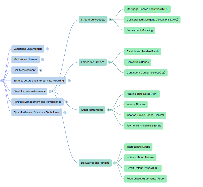
— Linden Lake

This series:
→　Topic Review (1 of 7): Fixed Income – Valuation Fundamentals
→　Topic Review (2 of 7): Fixed Income – Markets and Issuers
→　Topic Review (3 of 7): Fixed Income – Risk Measurement
→　Topic Review (4 of 7): Fixed Income – Term Structure and Interest Rate Modeling
→　Topic Review (5 of 7): Fixed Income – Fixed-Income Instruments
→　Topic Review (6 of 7): Fixed Income – Portfolio Management and Performance
→　Topic Review (7 of 7): Fixed Income – Quantitative and Statistical Techniques

References:
Reference 1, Reference 2, Reference 3