Topic Review (4 of 7): Fixed Income – Term Structure and Interest Rate Modeling

1. The Term Structure of Interest Rates as the Analytical Foundation

The term structure of interest rates represents the mathematical relationship between default-risk-free interest rates (or yields on zero-coupon bonds) and their times to maturity.

The Spot Curve: A series of yields-to-maturity on zero-coupon bonds. This curve represents the most fundamental benchmark for the time value of money because zero-coupon cash flows are entirely free of reinvestment risk.
Derivation via Bootstrapping: Spot curves are typically derived from the observable yields of liquid benchmark coupon bonds (such as on-the-run Treasury securities) using a step-by-step recursive process called bootstrapping.
The Forward Curve: A series of interest rates determined today for loans that will be initiated at a specific future date. Under no-arbitrage conditions, the spot, par, and forward curves contain identical information and can be translated directly into one another.
Active Management Implications: In an upward-sloping yield curve environment, if spot rates remain unchanged over an investment horizon, a bond will “roll down” the curve and trade at lower yields (and higher prices), earning a term premium. Active portfolio managers construct strategies based on their expectation that the actual future spot curve will differ from the path currently implied by the forward curve.

2. General Principles of Interest Rate Modeling

To value complex securities whose cash flows depend on the path of interest rates (such as callable/putable corporate bonds, mortgage-backed securities, and interest rate derivatives), simple spot-curve discounting is inadequate. Because future cash flows are contingent on rate paths, practitioners construct interest rate models—probabilistic, mathematical descriptions of how interest rates can evolve over time.

To implement these models numerically, analysts utilize lattices or trees:

Binomial Trees: A lattice where, at each discrete time step, the short-term interest rate can make one of two possible moves (an up-step or a down-step).
Trinomial Trees: A lattice where interest rates can take on one of three possible rates in the next period.
Recombination: Models typically assume that an up-step followed by a down-step yields the same rate as a down-step followed by an up-step. This recombining property prevents the tree from expanding exponentially, ensuring highly efficient computation.
Distributional Assumptions: Traditional models often utilize a lognormal random walk (or lognormal tree), which mathematically prevents interest rates from becoming negative and naturally models higher interest rate volatility at higher rate levels. However, negative-rate regimes in international markets have historically challenged strict lognormal constraints.

3. Classification of Term Structure Models

The fixed-income literature classifies term structure models into two primary categories:

A. Equilibrium Models

Equilibrium models seek to describe term structure dynamics using fundamental economic variables assumed to dictate interest rates, establishing pricing frameworks for bonds and options under an economic equilibrium. These are usually one-factor models where the single driving factor is the short-term interest rate (r).

The Cox-Ingersoll-Ross (CIR) Model: Incorporates mean reversion to drag the short-term rate toward a long-term target (b). Notably, it models interest rate volatility as proportional to the square root of the rate ( $\sigma\sqrt{r}$ ), which mathematically prevents rates from turning negative.
The Vasicek Model: Also incorporates mean reversion, but assumes that interest rate volatility remains constant. A notable drawback of the Vasicek model is that it is theoretically possible for interest rates to become negative.
Limitation: Because equilibrium models rely on a small number of constant parameters, they cannot be calibrated to perfectly match the currently observed market yield curve. Consequently, they may generate prices for option-free benchmark bonds that are inconsistent with actual market prices.

B. No-Arbitrage (Arbitrage-Free) Models

To overcome the pricing mismatches of equilibrium models, arbitrage-free models are calibrated using the observed market prices of a reference set of benchmark bonds. They allow model parameters to vary deterministically over time, ensuring that the model-derived prices of option-free benchmark bonds match current market prices exactly.

Ho-Lee (HL) Model: The first arbitrage-free model. It is a normal model with a time-dependent drift, meaning that interest rates are symmetrical and can theoretically become negative. It does not incorporate mean reversion, and volatility is independent of the rate level.
Kalotay-Williams-Fabozzi (KWF) Model: A log-normal analogue of the Ho-Lee model. Because the natural logarithm of the short rate follows a normal process, the rate itself remains strictly positive, though it lacks mean reversion.
Black-Derman-Toy (BDT) Model: A log-normal model that is capable of capturing a realistic term structure of interest rate volatilities. It introduces mean reversion endogenously; mean reversion is driven entirely by the slope of the local volatility curve over time.
Hull-White (HW) Model: An extension of the Ho-Lee model that explicitly models mean reversion, specifying both a central tendency and the speed at which the short rate reverts to it. It is a normal-rate model often implemented via a trinomial lattice.
Black-Karasinski (BK) Model: The logarithmic analogue of the Hull-White model. It explicitly models mean reversion, but because it is lognormal, interest rates are mathematically restricted from becoming negative.

4. Advanced Term Structure Modeling: The Gauss+ Model

While classical models are often single-factor (where the short rate is the only stochastic variable driving all maturities), complex cross-term hedging and curve trading require more advanced frameworks.

The Gauss+ Model is a popular multi-factor model utilized by practitioners for relative value and macro-style trading:

Three Cascade Factors: The model defines three factors: a short-term rate (r), a medium-term factor (m) representing business cycles and monetary policy expectations, and a long-term factor (l) reflecting long-run real rate and inflation expectations.
Mean Reversion Structure: The short-term rate mean reverts to the medium-term factor, which in turn reverts to the long-term factor, which itself reverts slowly to a long-run constant target (μ).
Pegging Short-Rate Volatility: In the risk-neutral dynamics, the equation for the short rate (dr) has no random volatility shock. This design mirrors real-world central bank policy (where policy rates are pegged at target levels and adjusted discretely) and enables the model to successfully capture the empirically observed hump-shaped term structure of yield volatility (where volatility is low at the very short end before rising at intermediate tenors).

5. Impact of Model Assumptions on Option-Adjusted Spread (OAS) and Risk Metrics

The selection of an interest rate model has profound mathematical consequences on the pricing and risk sensitivities of bonds with embedded options.

Option-Adjusted Spread (OAS): The constant spread that, when added to every rate in the interest rate tree, equates the model’s theoretical price to the actual market price of the security.
Distributional Impact: Normal-interest-rate models (e.g., Ho-Lee and Hull-White) systematically produce higher OAS estimates than lognormal models (e.g., KWF, BDT, and Black-Karasinski). This is because normal models allow for negative rates, which increases the probability of extreme low-rate states, thereby altering the option’s value and inflating the calculated spread.
Volatility Sensitivity: In a pricing tree, higher assumed volatility increases the value of embedded options. For a callable bond (long straight bond minus an issuer call option), higher volatility increases the call option’s value, lowering the callable bond’s price and compressing its OAS. For a putable bond (long straight bond plus an investor put option), higher volatility increases the put option’s value, raising the bond’s price and its OAS.
Effective Duration and Convexity: Effective duration and effective convexity must be calculated using full instrument repricing across the lattice after shifting the benchmark curve up and down. The lognormal models yield effective convexity patterns that are highly representative of actual pricing behavior, capturing where effective convexity turns negative (concave) for callable bonds when rates decline and the call option moves near or into the money.

Yield Curve Dynamics

1. The Three Principal Components of Yield Curve Dynamics

Empirical studies of major sovereign bond markets have demonstrated that changes in the yield curve are rarely perfectly parallel. Instead, yield curve dynamics are dominated by nonparallel shifts. To make sense of these complex movements, practitioners utilize Principal Component Analysis (PCA), a statistical technique that reduces observed historical yield curve changes to a combination of three independent synthetic factors:

Level (Factor 1 / PC1): Traditionally represents an approximately parallel shift up and down across the entire length of the yield curve. This is universally the most critical factor, explaining between 77% (Litterman and Scheinkman) and 92% (Phoa) of historical yield curve variance.
Steepness/Slope (Factor 2 / PC2): Represents a nonparallel change in the slope of the curve, where short-term rates and long-term rates move in contrary directions. This factor explains approximately 5% to 17% of the total curve variance.
Curvature/Twist (Factor 3 / PC3): Reflects a change in the “hump” of the curve, where yields at the short- and long-term maturities rise (or fall) while intermediate-term yields fall (or rise). It generally accounts for 1% to 3% of the overall variance.

A linear combination of these three independent principal components explains between 97% and 98.5% of all observed historical yield curve changes.

In terms of yield volatility, the term structure typically slopes downward. Short-term rates are empirically much more volatile than long-term rates because short-term yields are highly sensitive to central bank monetary policy actions and uncertainty. In contrast, long-term yields are anchored by slower-moving expectations of the real economy and long-term inflation. Furthermore, cross-country PCA reveals that while these three factors are universal, the “level” shift is less dominant in countries like Canada, the UK, Germany, and Japan compared to the US, implying that simple parallel duration does a poorer job of capturing interest rate risk in those international markets.

2. The Core Curves of the Term Structure

In fixed-income mathematics, the term structure of interest rates is formally represented by three highly interrelated curves. Under no-arbitrage rules, if any one of these curves is known, the other two can be mathematically derived:

The Spot Curve: A sequence of annualized yields-to-maturity on default-free zero-coupon bonds. Since zero-coupon bonds have no periodic coupons, the spot curve represents the “pure” time value of money completely free of reinvestment risk.
The Par Curve: A sequence of yields-to-maturity on coupon-paying government bonds assuming they are priced exactly at par value.
The Forward Curve: A series of interest rates set today for loans or investments that will begin at specified future dates.

When the spot curve is upward sloping, the forward curve lies above the spot curve. This mathematical relationship is a reflection of a basic averaging truth: when the average (the spot rate) is rising, the marginal data point (the forward rate) must be above that average. Conversely, when the spot curve is downward sloping (inverted), the forward curve lies below the spot curve.

Active bond portfolio managers closely monitor the relationship between expected future spot rates and implied forward curves. If a manager expects future spot rates to be lower than the rates currently locked into the forward curve, they will purchase long-term bonds. In an upward-sloping, stable yield curve environment, this gives rise to a strategy known as “riding (or rolling down) the yield curve”. As the bond approaches maturity, it “rolls down” to shorter tenors, where it is valued at successively lower spot yields and thus higher prices, allowing the investor to sell the bond before maturity to realize capital gains.

3. Measuring and Managing Curve Risk

Traditional single-factor risk metrics, such as modified duration or money duration, assume that interest rates of all maturities shift by the exact same amount in a parallel fashion. However, because yield curves frequently steepen, flatten, or twist, portfolios with identical parallel durations can perform vastly differently. Managing this shaping risk requires multi-factor frameworks:

Key Rate Duration (Partial Duration): Measures the portfolio’s sensitivity to a small change in the spot rate at a specific key maturity segment on the benchmark curve while holding all other key rates constant. Popular key maturities align with highly liquid, on-the-run Treasury benchmarks (typically ranging from 3 months/6 months up to 30 years). The sum of all key rate durations is mathematically equal (or very nearly equal) to the portfolio’s total parallel effective duration.
Yield-Curve-Reshaping Durations: Focuses on specific segments of the curve, dividing interest rate risk into short-end duration (SEDUR) (driven by the 10-year to 2-year spread) and long-end duration (LEDUR) (driven by the 30-year to 10-year spread).
Level, Slope, and Curvature Durations: Rather than shifting arbitrary key rates, this approach models changes in portfolio value directly against the Level, Slope, and Curvature factors identified via principal component analysis.

4. Integration with Term Structure and Interest Rate Modeling

To value complex bonds—specifically those with interest-rate-sensitive cash flows (e.g., corporate bonds with embedded call/put options, or prepayable mortgage-backed securities)—practitioners cannot rely on static spot curves. They must model how interest rates can vary randomly over time using stochastic interest rate models. These are typically implemented numerically via recombining binomial or trinomial interest rate trees/lattices:

Modern term structure models are classified into two primary categories:

A. Equilibrium Models

These models describe interest rate dynamics using fundamental economic variables to establish a pricing equilibrium for bonds and derivatives. They are typically single-factor models driving the instantaneous short rate, .

The Cox-Ingersoll-Ross (CIR) Model: Specifies that the short rate is mean reverting. Crucially, it models local interest rate volatility as proportional to the square root of the short rate ( $\sigma\sqrt{r}$ ), which mathematically prevents interest rates from becoming negative.
The Vasicek Model: Also assumes mean reversion, but models interest rate volatility as a constant. Because volatility does not scale down with the interest rate level, it is theoretically possible for interest rates to become negative under the Vasicek model.
Limitation: Because equilibrium models have only a finite number of parameters, they cannot be calibrated to perfectly match the currently observed market yield curve, meaning they can generate theoretical prices for benchmark option-free bonds that differ from actual market prices.

B. Arbitrage-Free (No-Arbitrage) Models

These models take the currently observed market term structure as given and price options and other derivatives relative to it. By using a time-dependent drift parameter, they are calibrated so that model-derived bond prices match current market prices exactly.

The Ho-Lee Model: The first arbitrage-free model. It models the short rate as a normal process with time-dependent drift and constant volatility, meaning negative rates are possible.
The Kalotay-Williams-Fabozzi (KWF) Model: A lognormal analogue to Ho-Lee; by modeling the natural log of the short rate, the short rate itself is restricted to positive values (though it lacks mean reversion).
The Black-Derman-Toy (BDT) Model: A lognormal model that captures a realistic term structure of interest rate volatilities. It introduces mean reversion endogenously through the shape of the local volatility curve over time.
The Black-Karasinski (BK) Model: A lognormal model that explicitly incorporates mean reversion.
The Hull-White (HW) Model: A normal-rate model that explicitly incorporates mean reversion, typically implemented via a trinomial lattice.
The Gauss+ Model: A highly popular multi-factor term structure model utilized for relative value and macro-style trading. It models three cascading factors: the short-term rate (, representing central bank policy), a medium-term factor (, reflecting business cycles and monetary expectations), and a long-term factor (, reflecting long-run real rates and inflation). Significantly, the Gauss+ model excludes a random volatility shock from the short-rate equation, allowing it to mimic discrete central bank pegging and accurately capture the empirically observed hump-shaped term structure of yield volatility (where volatility starts low at the very short end before rising at intermediate tenors).

5. Impact of Lattices on Embedded Options and Risk Sensitivities

The choice of interest rate model and volatility assumptions directly dictates the pricing and calculated risk metrics of option-embedded securities:

Option-Adjusted Spread (OAS): The constant spread added to every rate in the interest rate tree to equate the model’s theoretical price to the market price. Lognormal term structure models systematically yield lower OAS estimates than normal models because normal models allow for negative rate states, which inflates the theoretical option value and consequently pushes up the calculated risk spread.
Effective Duration and Convexity: For bonds with embedded options, traditional modified duration fails because changes in interest rates alter the expected cash flows. By shifting the benchmark curve up and down, reconstructing the interest rate tree, and keeping the OAS constant, models calculate effective duration.
- For callable bonds, as interest rates fall and the call option moves near or into the money, the potential price appreciation is capped. This price compression causes the effective duration to shorten dramatically and the effective convexity to turn negative (concavity).
- For putable bonds, as interest rates rise, the put option moves into the money, establishing a price floor. This limits price depreciation and shortens the effective duration while keeping the effective convexity positive.

Parallel Shifts

1. Definition and Mathematical Role of Parallel Shifts

In fixed-income mathematics, a parallel shift is defined as a yield curve movement in which interest rates or yields across all maturities change by the exact same number of basis points in the same direction.

Because of its mathematical simplicity, the parallel-shift assumption serves as the primary foundation for classical risk measurement. Traditional yield-duration statistics—such as Macaulay duration, modified duration, and money duration—inherently assume a parallel shift in a bond’s own yield. Similarly, effective duration (a curve duration statistic) measures the percentage change in a bond’s price given a parallel shift across the entire benchmark yield curve (such as the government par curve).

Under these one-factor risk frameworks, parallel shifts are highly significant because they are the largest driver of price volatility, historically accounting for approximately 90% of the total change in a bond’s value.

2. The “Level” Factor in Yield Curve Dynamics

When analysts study empirical yield curve movements using Principal Component Analysis (PCA), the parallel shift is mathematically identified as the first principal component, commonly referred to as the “level” factor.

This empirical research confirms the structural dominance of parallel movements:

Explanatory Power: Across major sovereign bond markets, the “level” shift is universally the most critical component, explaining between 77% and 92% of historical yield curve variance.
Volatility Trends: In a risk-neutral world, a parallel shift indicates that expectations of inflation, monetary policy, and economic growth have shifted uniformly. However, because long-term rates are anchored by slow-moving structural expectations while short-term rates are highly sensitive to central bank policy, true parallel shifts are rare over longer horizons.

3. Limitations of the Parallel Shift Assumption

While convenient, relying strictly on the parallel shift assumption introduces severe vulnerabilities in credit and portfolio risk management:

Failure of Single-Factor Hedges: Real-world yield curve shifts are rarely perfectly parallel. Instead, curves steepen, flatten, or twist. Hedges constructed using parallel-shift metrics (such as a standard ratio of DV01s) often fail to perform reliably when nonparallel movements occur.
Performance Divergence (Barbell vs. Bullet): Two portfolios can be structured to have the exact same duration matching a parallel shift. However, under nonparallel shifts, their performance diverges dramatically. For instance, in a steepening yield curve scenario, a concentrated bullet portfolio will outperform a duration-matched barbell portfolio. Conversely, in a flattening scenario, the barbell portfolio will outperform.
Empirical Rejection: In active trading, regressing daily yield changes of corporate bonds against Treasury benchmarks consistently rejects the parallel shift hypothesis. Corporate bonds trade at a credit spread that fluctuates independently of risk-free yields, meaning corporate and government curves do not move in a parallel, lockstep fashion.
The Level Factor’s Shorter-Term Imperfections: Even the PCA “level” component itself is not perfectly parallel across all maturities. In empirical USD swap markets, the level factor is not particularly level for shorter maturities between one and seven years, where central bank pegging dampens volatility.
International Discrepancies: The dominance of parallel movements is country-specific. Studies demonstrate that the first principal component (the level shift) is significantly less dominant in Canada, the United Kingdom, Germany, and Japan compared to the United States. Consequently, relying on parallel duration to manage interest rate risk does a poorer job in those international markets.

4. Decomposing Parallel Risks to Manage “Shaping Risk”

To overcome the blind spots of the parallel shift assumption, modern fixed-income mathematics decomposes parallel exposure into multi-factor risk measures designed to identify shaping risk.

By abandoning the assumption that all maturities move in parallel, portfolio managers utilize:

Key Rate Durations (Partial Durations): Shifting individual maturity segments on the benchmark curve one at a time while holding other rates constant. The sum of a portfolio’s key rate durations reconstructs its total parallel duration, allowing managers to see exactly where their curve risk is concentrated.
Yield-Curve-Reshaping Durations: Isolating sensitivity specifically to short-end steepening/flattening (SEDUR) versus long-end shifts (LEDUR).
Forward-Bucket ’01s: Directly shifting independent forward-rate segments (or “buckets”) of the curve to analyze localized cash-flow vulnerabilities.

Twists (Steepness)

In the larger context of yield curve dynamics, a twist is defined as a nonparallel term structure movement in which interest rates at different maturities move in contrary directions. This stands in contrast to a parallel shift, which assumes interest rates across all maturity segments change by the exact same amount in the same direction. Because interest rates of different terms rarely move in perfect sync, managing this nonparallel exposure—commonly referred to as shaping risk—is a core focus of fixed-income portfolio management and risk measurement.

1. Principal Component Analysis (PCA) and the “Slope” Factor

To understand yield curve movements, researchers use Principal Component Analysis (PCA) to decompose historical interest rate changes into three independent synthetic factors: level, steepness (slope), and curvature.

Within this statistical framework, the twist or change in steepness is established as the second principal component (PC2):

Explanatory Power: While parallel “level” shifts explain the vast majority of yield curve variance, the “slope” or “steepness” factor is the second most critical driver, explaining between 5% and 17% of historical yield curve variance depending on the time period and sovereign market.
Directional Movement: A unitary positive standard deviation change in the slope factor typically raises yields at shorter maturities while lowering yields at longer maturities, or vice versa. This factor captures the nonparallel steepening or flattening of the yield curve.

These slope changes are categorized into two primary market environments:

Steepening: Occurs when long-term interest rates increase relative to short-term rates (for example, if short-term rates stay flat or decline while long-term rates rise significantly).
Flattening: Occurs when short-term interest rates increase relative to long-term rates (for instance, if short-term rates rise while long-term rates drop or remain flat).

2. Decomposing Twists in Performance Attribution

Because traditional duration measures assume parallel yield curve shifts, they cannot capture how twists affect the actual returns of a portfolio. To evaluate a manager’s performance, advanced holdings-based attribution models explicitly isolate the return generated by these twists:

The Kahn Multifactor Model: This model decomposes yield curve movements into three distinct factors, defining a twist specifically as a term structure change where short-term rates increase by a certain number of basis points (), intermediate rates remain unchanged, and long-term rates decrease by that same .
The Campisi Attribution Model: In an extended Campisi framework, the overall risk-free Treasury return is decomposed into a shift return and a twist return. The shift return is calculated by multiplying the portfolio’s starting duration by the parallel yield change of a maturity-matched key-rate benchmark. The twist return is then isolated as the portion of the Treasury return that cannot be explained by this parallel shift, capturing the exact return contribution of the curve’s nonparallel reshaping.

3. Measuring and Managing Twist and Shaping Risks

To defend portfolios against the volatility of curve twists, fixed-income managers utilize multi-factor risk measures to map and hedge their exposures:

Key Rate Durations (Partial Durations): This popular approach measures the sensitivity of a bond or portfolio’s price to a small interest rate shift at a specific maturity segment of the curve (e.g., 2-year, 5-year, 10-year, or 30-year segments) while holding all other spot rates constant. Summing a portfolio’s key rate durations yields its total parallel effective duration, but analyzing them individually allows managers to see their exposure to steepening or flattening curves.
Yield-Curve-Reshaping Durations: Rather than shifting individual key rates, this framework simplifies curve exposure by measuring a portfolio’s sensitivity directly at the short and long ends of the curve relative to a 10-year benchmark. It calculates Short-End Duration (SEDUR), representing price sensitivity to changes in the 10-year to 2-year spread, and Long-End Duration (LEDUR), representing price sensitivity to changes in the 30-year to 10-year spread.
Level, Slope, and Curvature Durations: This method fits the yield curve to a mathematical function. For example, in the Willner model, the slope of the yield curve is captured by the parameter ratio (where is the estimated spread between long- and short-term rates, and is maturity), allowing managers to calculate and hedge their portfolio’s direct sensitivity to slope changes.

Butterfly Movements (Curvature)

In the mathematical and statistical framework of fixed-income analysis, curvature (or butterfly) movements represent the third most significant type of yield curve shift. Empirical studies utilizing Principal Component Analysis (PCA) reveal that after accounting for parallel level shifts (the first principal component, which explains 77% to 92% of yield curve variance) and steepness/slope twists (the second principal component, explaining 5% to 17%), curvature shifts (the third principal component) explain a small but vital 1% to 3% of historical yield curve fluctuations.

1. Mathematical and Statistical Mechanics of Curvature

Curvature movements capture nonparallel shifts where different maturity segments of the yield curve move in contrary, non-linear directions:

The Curvature Shift Profile: Economically, a standard curvature or “butterfly” shift describes a scenario where both short-term and long-term interest rates move in one direction, while intermediate-term (medium-term) interest rates move in the opposite direction. For example, in a positive curvature shift, short- and long-term rates rise while intermediate rates fall.
The “Hump” and Peak Maturity: Curvature represents a change in the “hump” of the yield curve. Under classical PCA models, the peak of this hump is typically located around the 10-year maturity segment.
The Kahn Attribution Definition of a Butterfly Shift: Within holdings-based performance attribution, such as the Kahn multifactor model, a butterfly shift is contractually defined as a specific term-structure movement where both short-term and long-term rates increase by basis points, while intermediate (medium-term) rates simultaneously decrease by 24 basis points.

2. Parametric Modeling of Curvature

To quantify these dynamics, modern term structure modeling incorporates curvature as an explicit variable:

The Willner Model: In parametric curve-fitting, the yield curve is represented mathematically as a function:

where Y is the yield to maturity, M is the maturity in years, H is a constant determining the curve’s hump positioning, and C represents the curvature of the yield curve.

The Short-Rate PC (Curvature): In PCA modeling of swap curves, the third principal component—often referred to as the short-rate or curvature factor—reflects a simultaneous small increase in very short-term rates, a small decrease in intermediate-term rates, and a small increase in long-term rates.

3. Managing Curvature and Butterfly Risk in Portfolio Strategies

Traditional single-factor risk measures, such as modified duration, assume parallel yield curve shifts and fail to measure shaping risk. Managing exposure to curvature and butterfly twists requires more advanced, multi-factor risk measures:

Key Rate Durations (KRD): This approach measures a portfolio’s price sensitivity to a small change in the spot rate at a specific key maturity segment of the benchmark curve (typically across 11 key maturities from 3 months to 30 years) while holding all other rates constant.
Level, Slope, and Curvature (LSC) Durations: This method directly measures a portfolio’s interest rate sensitivity to the individual parameters of a fitted mathematical yield curve (such as the C parameter in the Willner model).
The Bullet vs. Barbell Conflict: Curvature shifts are the primary driver of performance dispersion between bullet portfolios (which concentrate maturities around a single intermediate point) and barbell portfolios (which split maturities between short-term and long-term extremes). Even if a bullet portfolio and a barbell portfolio are structured to have the exact same total parallel duration, a positive butterfly shift (where short-term and long-term rates rise while intermediate-term rates fall) will cause the bullet portfolio to dramatically outperform the barbell portfolio. Managing the key rate and curvature durations allows portfolio managers to hedge against or actively exploit these nonparallel shaping risks.

Term Structure Theories

Traditional term structure theories offer qualitative frameworks to explain the economic forces that shape the yield curve, describing how market expectations, risk premiums, and institutional constraints determine interest rates across different maturities. In the broader context of fixed-income analysis, these traditional theories provide the conceptual foundation that modern, quantitatively precise interest rate models (such as equilibrium and arbitrage-free models) mathematically operationalize to price complex securities and manage risk.

The sources outline four traditional theories of the term structure, alongside their integration into modern financial modeling:

1. Traditional Term Structure Theories

A. Expectations Theories (Pure vs. Local)

Expectations-based theories interpret the shape of the yield curve primarily through investors’ expectations of future interest rates:

Pure (or Unbiased) Expectations Theory: This theory asserts that the forward rate is an unbiased predictor of the future spot rate. It assumes that investors are risk-neutral, meaning bonds of any maturity are perfect substitutes for one another, and any investment strategy over a given horizon will yield the same expected return.
Local Expectations Theory: This theory adapts expectations theory to a world characterized by risk. While it assumes risk-neutrality over a very short holding period—holding that the expected return of any long-term bond over one period is exactly equal to the one-period risk-free rate—it places no such restrictions on longer-term investment horizons.

B. Liquidity Preference Theory

This theory rejects the assumption of risk neutrality, asserting that investors are risk-averse and prefer short-term, liquid securities.

Because longer-term bonds carry greater price sensitivity to interest rate changes (duration risk), investors demand a liquidity premium (or term premium) to induce them to lend long-term.
Under this theory, forward rates are an upwardly biased estimator of expected future spot rates because they incorporate this positive premium.
While the presence of liquidity premiums means the yield curve is typically upward-sloping, a downward-sloping (inverted) yield curve can still occur if market expectations of deflation or falling spot rates are strong enough to override the positive liquidity premium.

C. Segmented Markets Theory

The segmented markets theory focuses on institutional constraints, such as regulatory or self-imposed asset-liability management (ALM) policies.

It assumes that market participants are unwilling or unable to invest in maturities outside of their preferred sector to avoid asset-liability mismatch risks (e.g., life insurers and pension funds naturally operate in the long end of the curve, while money market funds are restricted to short-term instruments).
Consequently, each maturity sector acts as an independent market, and the yield of a given maturity is determined strictly by the localized supply and demand for funds within that segment, completely divorced from expectations or liquidity premiums.

D. Preferred Habitat Theory

This theory reconciles expectations and segmented market dynamics. It acknowledges that borrowers and lenders have strong maturity preferences (habitats) dictated by their liabilities, but rejects the idea that maturity segments are completely independent. Instead, it posits that market participants are willing to cross over into different maturity sectors if they are offered a sufficient yield or return premium to compensate for the additional risk.

2. The Larger Context: Traditional Theories vs. Modern Modeling

While traditional theories provide essential economic intuition, modern term structure modeling bridges these qualitative concepts with rigorous mathematical implementation to price bonds and derivatives:

Quantitative Precision: Traditional theories are primarily conceptual and descriptive. Modern models use stochastic differential equations (SDEs) to generate random paths of interest rates over time, implementing recombining binomial or trinomial lattices to price options and interest-rate-contingent cash flows.
Risk-Neutral Pricing & Indistinguishability: In modern term structure modeling, expectations and risk premiums are often modeled together. Under the risk-neutral pricing framework, it is impossible to separate rate expectations from the risk premium based on a cross-section of bond prices alone. This is because a drift term in a model’s rate equation (such as in the Vasicek or CIR models) can mathematically represent either an expected short-rate change or a risk premium. Modern practitioners focus on the risk-neutral process because it is what directly dictates the market-clearing prices of assets.
The Analytical Decomposition of Forward Rates: Modern continuous-time term structure models formally decompose the forward rate curve (f(T)) into three specific, identifiable components:

This formula integrates expectations (the short rate plus expected rate changes scaled by duration D ), the risk premium ( λ scaled by duration), and a negative convexity adjustment (arising from interest rate volatility σ2 and bond convexity C ). Under the pure expectations hypothesis of traditional theory, λ=0. Under the pure risk premium hypothesis, expectations of rate changes are zero (E[dr/dt]=0). In reality, modern financial engineering models the yield curve as a dynamic combination of all three elements.

Pure Expectations

The Core Premise of Pure Expectations Theory

In the study of the term structure of interest rates, pure expectations theory (historically also known as unbiased expectations theory) asserts that the shape of the yield curve is exclusively determined by market expectations of future interest rates.

Under this hypothesis:

No Risk Premium: The risk premium (λ) is assumed to be exactly zero (λ=0).
Unbiased Predictors: Implied forward rates are completely unbiased predictors of future short-term spot rates.
Perfect Substitutes: Bonds of different maturities are treated as perfect substitutes for one another.
Equal Expected Returns: Any investment strategy over a given horizon is expected to yield the same return. For example, buying a five-year bond and holding it for three years will yield the exact same expected return as buying a three-year bond outright, or rolling over a series of three consecutive one-year bonds.
The “No-Change” Baseline: If spot rates evolve exactly as the forward curve implies, a total return investor will earn the first-period risk-free spot rate regardless of the maturity of the bond they purchase.

Economic Assumptions

The pure expectations theory relies fundamentally on the assumption of risk neutrality. In a risk-neutral world, investors are entirely unaffected by uncertainty, which means risk premiums do not exist, and every debt security yields the risk-free rate of return associated with its specific maturity.

The Larger Context of Term Structure Theories

Traditional term structure theories attempt to explain why yield curves take on various shapes (such as upward-sloping, flat, humped, or inverted) by adjusting or rejecting the strict assumptions of pure expectations:

1. Pure Expectations vs. Local Expectations Theory

The local expectations theory is a more mathematically rigorous offshoot of expectations-based modeling. While pure expectations claims that different maturity strategies will yield the same return over any investment horizon, local expectations restricts this risk-neutrality to short holding periods. It contends that the expected return of any bond (even a risky or long-term bond) over the next immediate short-term period is equal to the risk-free rate, leaving room for risk premiums to exist over longer-term horizons.

2. Pure Expectations vs. Liquidity Preference Theory

The liquidity preference theory rejects the assumption of risk neutrality, asserting that investors are risk-averse and require compensation for the interest rate risk inherent in holding longer-term securities. It posits that liquidity premiums exist and monotonically increase with a bond’s maturity. Because of these built-in premiums, forward rates are actually upwardly biased estimators of expected future spot rates, which directly refutes the “unbiased” claim of pure expectations.

3. Pure Expectations vs. Segmented Markets Theory

The segmented markets theory ignores expectations and liquidity premiums altogether, arguing that the yield curve is shaped entirely by the independent supply and demand of funds within separate maturity sectors. Because of self-imposed or regulatory asset-liability management (ALM) constraints, institutions are assumed to be unwilling or unable to cross over into other maturity segments (e.g., life insurers and pension funds naturally operate at the long end of the curve, while money market funds are restricted to the short end).

4. Pure Expectations vs. Preferred Habitat Theory

The preferred habitat theory bridges the gap between expectations and segmented markets. It agrees that institutions have strong maturity preferences (habitats) dictated by their liabilities, but asserts that they are willing to deviate from their preferred maturities if they are offered a sufficient yield premium to justify taking on the additional risk.

Empirical Reality and Limitations

The sources emphasize that the pure expectations hypothesis is empirically refuted by market evidence. In actual markets:

Risk premiums and liquidity premiums do exist, meaning forward rates consistently act as upwardly biased estimators rather than unbiased predictors.
Even the short-horizon predictions of the local expectations theory fall short; historical data demonstrates that short holding-period returns on long-dated bonds are generally higher than those on short-dated risk-free bonds, reflecting the risk-return trade-off expected by risk-averse investors.

Liquidity Preference

Core Premise of Liquidity Preference Theory

Unlike the pure expectations theory, which assumes investors are risk-neutral, liquidity preference theory attempts to account for risk aversion. The theory asserts that liquidity premiums exist to compensate investors for the added interest rate risk they face when lending long-term.

The mechanics of this premium are rooted in the investment horizon and price sensitivity:

The Price Risk of Longer Maturities: Because the majority of investors have an investment horizon that is shorter than the maturity of long-term bonds (such as a 30-year Treasury), they face the risk that the yield curve will change and force them to sell prior to maturity at an uncertain price. Lenders demand an incrementally higher return—the liquidity premium—to induce them to take on this price risk.
A Crucial Distinction on “Liquidity”: The term “liquidity premium” in this context is a maturity premium applying to all long-term bonds, even those with deep, active markets. It is not to be confused with a transaction-cost or yield premium that thinly traded bonds bear due to a lack of market-making depth.
Monotonic Increase: The theory posits that these liquidity premiums increase monotonically with maturity, meaning the premium for a longer maturity is always greater than or equal to that of a shorter maturity (LP(T+t)≥LP(T) for all t>0).

Impact on the Yield Curve and Forward Rates

Because of the compounding effect of the liquidity premium over time, the theory has distinct implications for the shape of the term structure and the predictive power of forward rates:

The Upward-Sloping Bias: If market participants expect future short-term spot rates to remain completely unchanged, the presence of monotonically increasing liquidity premiums means the yield curve will naturally exhibit an upward slope. Consequently, an upward-sloping yield curve is the “typical” state of the term structure.
Biased Forward Rates: Under this theory, forward rates are upwardly biased estimators of expected future spot rates. The forward rate equals the expected spot rate plus the biased addition of the liquidity premium, directly refuting the pure expectations hypothesis.
Accounting for Downward-Sloping Curves: Liquidity preference theory does not suggest that inverted yield curves are impossible. A downward-sloping yield curve can still occur under this framework if investors expect a severe decline in future spot rates or expect deflation (a negative rate of inflation due to monetary or fiscal policy actions). If the expected decline in spot rates is sharp enough, it will mathematically override and offset the positive effect of the liquidity premiums, causing the overall curve to slope downward.

The Larger Context of Traditional Term Structure Theories

To understand how liquidity preference fits into the broader qualitative landscape of fixed-income analysis, it must be contrasted with the other three traditional theories:

Pure (Unbiased) Expectations Theory: This theory operates under the assumption of complete risk neutrality. It argues that the risk premium is zero (λ=0), meaning bonds of all maturities are perfect substitutes and forward rates are completely unbiased predictors of future spot rates.
Local Expectations Theory: Similar to the pure expectations theory, this framework assumes risk neutrality, but strictly restricts it to short-term holding periods. It contends that the expected return of any bond over a very short time interval is the risk-free rate, but it allows for risk premiums to exist over longer-term investment horizons.
Segmented Markets Theory: This theory rejects the concept of expectations and liquidity premiums entirely. It assumes that borrowers and lenders are strictly confined to specific maturity sectors due to regulatory or self-imposed asset/liability management (ALM) constraints. Yields in each segment are determined independently by localized supply and demand, with no crossover between markets.
Preferred Habitat Theory: This theory bridges expectations and segmented markets. It acknowledges that institutions have strong maturity preferences (habitats) dictated by their liabilities, but rejects the idea that these markets are completely isolated. Instead, it asserts that investors will cross over into other maturity sectors if offered a sufficient yield premium to compensate for the deviation.

The Modern Quantitative Bridge

In modern continuous-time term structure modeling (such as the Vasicek and Gauss+ frameworks), these qualitative traditional concepts are unified and mathematically operationalized. Modern financial engineering models the instantaneous forward rate curve (f(T)) using an analytical decomposition:

This formulation unites expectations (the short rate plus expected rate changes scaled by duration D ), the risk premium ( λ scaled by duration, capturing the traditional liquidity premium concept), and a negative convexity adjustment (arising from interest rate volatility σ2 and bond convexity C). Under the traditional pure expectations hypothesis, the risk premium λ=0. Under the pure risk premium hypothesis (closely aligned with the liquidity preference baseline under flat expectations), the expected change in rates E[dr/dt]=0, meaning the shape of the curve is driven entirely by the risk premium. Importantly, modern modeling demonstrates that it is impossible to separate expectations of rate changes from the risk premium by observing a cross-section of bond prices alone, which is why practitioners calibrate their lattices using risk-neutral pricing.

Segmented Markets

1. The Core Premise of Segmented Markets Theory

Unlike expectations-based or liquidity preference theories, the segmented markets theory rejects the idea that interest rates across different maturities are mathematically linked by market expectations or risk premiums. Instead, it asserts that:

Independent Markets: Lenders and borrowers have rigid maturity preferences, meaning the yield curve is shaped entirely by the independent supply and demand for funds within each specific maturity segment. Each maturity bucket operates as a completely separate, isolated market.
Non-Substitutability: Debt instruments of different maturities are not substitutes for one another. Consequently, yields at one maturity are determined completely independently of the yields prevailing in other maturity segments.

2. Institutional Constraints and Asset-Liability Management (ALM)

The economic justification for segmented markets theory rests on the strict cash flow matching and asset-liability management (ALM) constraints faced by institutional market participants. To eliminate the risk of an asset-liability mismatch, major financial intermediaries restrict their investment activities exclusively to the maturity sector that directly aligns with their outstanding liabilities:

The Long End: Pension plans and life insurance companies naturally manage long-term liabilities. To avoid interest rate reinvestment risks (such as yields declining while the cost of their liabilities remains fixed), they restrict their activity as buyers to the long end of the bond market.
The Short End: Conversely, money market funds are legally or structurally constrained to short-term instruments, typically investing only in debt with a maturity of one year or less.

Because these institutions are assumed to be strictly unwilling (or unable) to cross over into other sectors, their localized supply and demand dictate the yield within those individual buckets.

3. The Larger Context of Term Structure Theories

To fully understand segmented markets theory, it must be contrasted with the other three traditional term structure frameworks:

A. Contrast with Expectations Theories (Pure and Local)

The unbiased (pure) expectations theory operates on the polar opposite assumption—that bonds of different maturities are perfect substitutes. It assumes investors are completely risk-neutral, meaning a portfolio’s return is driven entirely by expectations of future spot rates, and any combination of maturities over a given horizon will yield the same expected return. The local expectations theory also relies on perfect substitutability but limits this risk-neutrality to very short holding periods.

Segmented markets theory completely rejects this substitutability, arguing that institutional boundaries prevent any such seamless arbitrage across maturities.

B. Contrast with Liquidity Preference Theory

The liquidity preference theory assumes that investors are risk-averse and naturally prefer the short end of the curve because long-term bonds carry greater price volatility. Under this theory, forward rates are upwardly biased estimators of future spot rates because they must incorporate a monotonically increasing liquidity premium to induce investors to lend long-term.

Segmented markets theory, however, maintains that long-term yields can be low or high purely based on localized supply and demand dynamics, completely independent of a maturity-based “risk premium”.

C. Reconciliation via Preferred Habitat Theory

The preferred habitat theory serves as a direct bridge between the rigid segmentation of markets and expectations-based theories. It acknowledges that institutions have strong, liability-driven maturity preferences (“habitats”).

However, it rejects the idea that these markets are completely isolated. Instead, it posits that investors will cross over into other maturity segments if they are offered a sufficient yield premium to compensate them for taking on the additional asset-liability mismatch risk. By accepting elements of both the segmented markets theory and expectations-based theories, the preferred habitat theory is widely viewed by practitioners as a much more realistic description of real-world yield curve behavior.

Preferred Habitat

The Core Premise of Preferred Habitat Theory

The preferred habitat theory is a traditional term structure theory proposing that while many borrowers and lenders have strong maturity preferences (habitats) dictated by their asset-liability structures, they do not view different maturity segments as completely independent. In other words, unlike the segmented markets theory, it does not assert that yields at different maturities are determined completely in isolation.

Reconciling Expectations and Market Segmentation

Preferred habitat theory bridges the gap between the extreme assumptions of other traditional theories:

Segmented Markets Theory: Assumes that investors face rigid asset-liability management (ALM) or regulatory constraints that force them to strictly buy only the maturities that match their liabilities, rendering them entirely unable or unwilling to cross over into other maturity sectors.
Unbiased Expectations Theory: Assumes complete risk neutrality, meaning that bonds of different maturities are perfect substitutes and investors have no maturity preferences or habitats at all.

By contrast, the preferred habitat theory is built on the realistic economic premise that investors are risk-averse but can be induced to accept additional risk (such as asset-liability mismatches) if they are offered a sufficient yield or return premium. If a yield differential or expected return premium is large enough, institutions will gladly deviate from their preferred habitats:

Money Market Funds: Although they naturally prefer short-term, liquid instruments, they will lengthen the maturities of their assets if expected returns on longer-term securities exceed short-term rates by a wide enough margin.
Life Insurance Companies: Despite having long-term liabilities that draw them to the long end of the curve, they will stop limiting themselves to long-term bonds and place a portion of their funds in short-term investments if the return incentive on short-term debt becomes attractive enough.

Ultimately, the preferred habitat theory offers a more realistic explanation of real-world yield curves because it shows that both market expectations of future rates and institutional factors (such as liability-driven habitats) jointly determine the term structure of interest rates.

A Practical Application: Quantitative Easing (QE)

The sources demonstrate how preferred habitat dynamics operate in practice during unconventional monetary policy regimes, such as the Federal Reserve’s quantitative easing (QE) programs.

When the Fed launched QE, it purchased massive quantities of mortgage-backed securities (MBS) from the public, significantly shrinking the available supply of these assets. Many institutional MBS investors operate in a strict “preferred habitat” because they have invested substantial capital in gaining the highly specialized analytical skills required to manage the complex interest rate and prepayment risks unique to mortgage pools. Because these specialized institutions were unwilling or unable to easily exit the mortgage market and invest in other assets, the scarcity of supply forced them to bid aggressively against one another for the remaining MBS, which drove MBS yields down to historic lows.

Interest Rate Models

Fixed-income analytics require interest rate models to describe how interest rates can change over time . While traditional discounting using spot rates is sufficient for pricing option-free bonds , it is inadequate for valuing securities with embedded options (such as callable or putable corporate bonds and mortgage-backed securities) because their expected cash flows are interest-rate dependent . Interest rate models use stochastic differential equations (SDEs) to capture interest rate uncertainty mathematically and generate potential rate pathways .

1. Implementing Models Numerically via Lattices

To apply continuous SDEs in practice, these mathematical models are converted into discrete numerical lattices or trees .

Binomial Trees: At each discrete node, the short-term interest rate can make one of two possible moves (an up-step or a down-step) over a designated time step (such as six months or one year) .
Trinomial Trees: Allow interest rates to make one of three possible moves in the next period, offering an extra degree of freedom .
The Recombining Property: Most lattices are designed to recombine—meaning an up-step followed by a down-step yields the same rate as a down-step followed by an up-step . Recombination prevents the tree from expanding exponentially, ensuring faster, linearly scaling computations .

2. Equilibrium versus No-Arbitrage Models

Modern term structure models are broadly classified based on how they treat the current yield curve:

A. Equilibrium Models

These models describe interest rate dynamics using fundamental economic variables that are assumed to dictate interest rates, establishing pricing frameworks under an economic equilibrium . Because they rely on a small number of parameters, they cannot be calibrated to perfectly match the current market yield curve, meaning they can generate theoretical prices for benchmark option-free bonds that differ from actual market prices .

The Vasicek Model: Captures mean reversion to drag the short-term rate back toward a long-term target over time . It assumes interest rate volatility is constant, which introduces a major drawback: the short rate can theoretically become negative .
The Cox-Ingersoll-Ross (CIR) Model: Also assumes mean reversion, but models interest rate volatility as proportional to the square root of the rate ( $\sigma\sqrt{r}$ ) . This standard deviation factor ensures that interest rate moves shrink as rates approach zero, mathematically preventing negative rates .

B. No-Arbitrage (Arbitrage-Free) Models

These models take the observed market yield curve as given and allow parameters to vary deterministically over time to calibrate the interest rate tree so that model-derived bond prices match current market prices exactly . This calibration ensures the interest rate tree is consistent with the zero-coupon spot curve .

3. Key One-Factor Arbitrage-Free Models

The most common arbitrage-free models are one-factor models, where a single factor—typically the short-term interest rate—is assumed to drive all yield curve movements .

The Ho-Lee (HL) Model: The first arbitrage-free model, which assumes a normal process for the short rate (dr=θ(t)dt+σdz) . Because the rate is distributed normally and is unbounded, the short rate can become negative . It features constant local volatility and does not mean-revert .
The Kalotay-Williams-Fabozzi (KWF) Model: Directly analogous to the HL model, but it models the change in the natural logarithm of the short rate (ln(r)) . Because the rate follows a lognormal process (r=e_^ln(r)), the short rate itself can never become negative . Like the HL model, it lacks mean reversion .
The Black-Derman-Toy (BDT) Model: A lognormal process (dln(r)=[θ(t)+ρ(t)ln(r)]dt+σ(t)dz) that is capable of capturing a realistic term structure of interest rate volatilities . It introduces mean reversion endogenously; if the local volatility term structure is decreasing, the model exhibits mean reversion .
The Hull-White (HW) Model: A normal-rate process (dr=(θ−ϕr)dt+σdz) that explicitly models mean reversion, defining a central tendency and the speed at which the short rate reverts to it . This mean reversion reduces the probability of negative rates, although it does not eliminate it . It is often implemented on a trinomial tree .
The Black-Karasinski (BK) Model: The logarithmic analogue of the Hull-White model . It explicitly models mean reversion, and because it is lognormal, interest rates are mathematically restricted from becoming negative .

4. Multi-Factor Modeling: The Gauss+ Model

While one-factor models are computationally convenient, they assume that interest rates across all maturities are perfectly correlated and determined entirely by the short rate . Hedging complex portfolios across different parts of the curve requires multi-factor models .

The Gauss+ model is a three-factor model that defines a short-term rate (r, central bank policy), a medium-term factor (m, business cycle/monetary policy expectations), and a long-term factor (l, long-run economic growth/inflation expectations) . To reflect how central banks conduct policy, the equation for the short rate contains no random volatility shock (dr=−α_r(m−r)dt) . This design keeps short-rate volatility low, allowing the Gauss+ model to match empirically observed, hump-shaped term structures of volatility where volatility is low at the very short end before peaking at intermediate maturities .

5. Impact of Model Assumptions on Risk Metrics

The mathematical structure and distributional assumptions of an interest rate model directly dictate the calculated valuation and risk parameters of option-embedded securities:

Option-Adjusted Spread (OAS): The constant spread added to every rate in the interest rate tree to equate the model’s theoretical price to the market price . Normal models (such as Ho-Lee and Hull-White) systematically generate higher OAS estimates than lognormal models (such as KWF, BDT, and BK) . Because normal models allow for negative rate states, they inflate the theoretical option value of the embedded option, which in turn pushes up the calculated spread required to reconcile the model with the market price .
Effective Duration: Lognormal models produce effective duration estimates for callable and putable bonds that are highly sensitive to interest rate levels . In contrast, normal models (HL, HW) produce effective duration estimates that vary less across different rate levels .
Effective Convexity: Lognormal models generate convexity patterns that are highly representative of actual pricing behavior . For callable bonds, lognormal trees successfully capture the pricing behavior where effective convexity turns negative (concave) at intermediate rate levels as the call option moves near or into the money .

No-Arbitrage vs. Equilibrium

1. Conceptual and Philosophical Foundations

The choice between equilibrium and no-arbitrage (arbitrage-free) models represents a fundamental divide in how financial economists and practitioners approach the stochastic modeling of interest rates using stochastic differential equations (SDEs).

Equilibrium Models: These frameworks (such as the classic Vasicek and Cox-Ingersoll-Ross [CIR] models) are built on macroeconomic principles. They seek to describe the dynamics of the entire term structure by modeling a small set of fundamental economic variables—most commonly the instantaneous short-term interest rate (r))—assumed to dictate interest rates in a general market equilibrium. These models describe how the short rate evolves under real-world economic forces, such as mean reversion to a long-run equilibrium rate.
No-Arbitrage Models: In contrast, no-arbitrage models (such as the Ho-Lee, Hull-White, and Black-Derman-Toy models) are market-calibrated. They do not attempt to explain why the yield curve is shaped the way it is based on macroeconomic variables; instead, they take the currently observed market term structure as given. Because of this starting assumption, these models are often classified by theorists as “partial equilibrium” models. They focus strictly on defining a mathematically consistent, risk-neutral process that prevents any relative arbitrage opportunities from existing between different points on the curve.

2. The Calibration Trade-Off: Fitting the Current Curve

The most critical mathematical and practical distinction between these two modeling categories lies in their capacity to fit observable market prices:

The Inconsistency of Equilibrium Models: Because equilibrium models rely on a finite number of constant parameters (such as the speed of mean reversion a, the long-run rate b, and volatility σ), they lack the mathematical flexibility to perfectly match the currently observed market yield curve. When an equilibrium model is used to estimate the term structure, the model-derived yield curve will almost certainly deviate from actual market yields. Consequently, an equilibrium model will generate theoretical prices for option-free benchmark bonds that differ from their actual, observed market prices.
The Exact Fit of Arbitrage-Free Models: No-arbitrage models overcome this limitation by allowing their pricing parameters—specifically the drift term (θ_t)—to vary deterministically over time. By letting these parameters adapt to the market on a day-to-day basis, the interest rate lattice or tree is calibrated so that its model-derived benchmark bond prices match actual market prices exactly. This ensures that the model is perfectly consistent with the current par yield curve or zero-coupon spot curve.

3. Practical Usage and Practitioner Preferences

In the larger context of risk measurement and derivative pricing, these differences dictate how and when each model type is deployed:

Derivative and Option Valuation: For pricing interest rate derivatives (such as caps, floors, and swaptions) and bonds with embedded option features (such as callable or putable corporate debt), practitioners strongly prefer arbitrage-free models. Because these models guarantee that the underlying option-free benchmark bonds are priced exactly to market, they create a unified, consistent framework. If an equilibrium model is used instead, the pricing discrepancies on the underlying straight debt will distort the value calculated for the embedded option, producing unreliable valuation and risk metrics.
Identifying Market-Wide Mispricings: While equilibrium models are poorly suited for pricing contingent claims, they possess a distinct advantage in relative-value and active portfolio management. Because an equilibrium model is not “force-fitted” to match the market, it acts as an independent baseline of fair value. If a portfolio manager believes the model’s underlying economic assumptions and estimated parameters are correct, any deviation between the model’s yield curve and the actual market yield curve can be interpreted as a genuine market mispricing to be actively exploited.

One-Factor Models (Ho-Lee, BDT, Hull-White)

The Context of One-Factor Models in Interest Rate Modeling

In fixed-income mathematics, interest rate models provide a probabilistic description of how interest rates can change over time. Capturing this uncertainty is crucial because the cash flows of securities with embedded options or interest-rate derivatives depend directly on future rate pathways. These dynamics are mathematically formulated using stochastic differential equations (SDEs).

Within this broader framework, models are primarily categorized along two dimensions:

One-Factor vs. Multifactor Models: One-factor models assume that a single state variable—specifically the short-term interest rate (the “short rate,” r )—drives the changes in interest rates across all other maturities in the term structure. While they assume perfect correlation among yields and cannot capture shaping risks (such as steepening or twists), they are widely used because they are computationally efficient, and empirical studies show that a single parallel “level” shift accounts for more than 90% of yield curve changes.
Equilibrium vs. No-Arbitrage Models: Equilibrium models (such as the CIR or Vasicek models) derive interest rate behavior from macroeconomic variables but have a major limitation: they rely on a small set of constant parameters and cannot be calibrated to perfectly fit the current yield curve. In contrast, no-arbitrage (arbitrage-free) models take the observed market yield curve as given. By allowing their drift parameters to vary deterministically over time, they are calibrated to match the prices of option-free benchmark bonds exactly, creating a consistent framework to value derivative contracts and embedded options.

To implement these continuous SDE models numerically, practitioners convert them into discrete recombining lattices or trees (usually binomial or trinomial). Recombination enforces that an up-step followed by a down-step yields the same rate as a down-step followed by an up-step, keeping the tree’s growth linear rather than exponential, which drastically reduces computational complexity.

Detailed Analysis of Key One-Factor Arbitrage-Free Models

The Ho-Lee, Black-Derman-Toy (BDT), and Hull-White models represent distinct mathematical approaches to modeling the risk-neutral evolution of the short-term rate:

1. The Ho-Lee (HL) Model

Introduced in 1986, the Ho-Lee model was the first arbitrage-free interest rate model.

Mathematical SDE: It assumes a normal process for the short rate, specified as:

dr = θ(t)dt + σ(t)dz

where θ(t) is the time-dependent drift calibrated to the initial term structure, and is the local volatility of the short rate.

Volatility & Mean Reversion: The volatility of the short rate is constant and independent of the rate level. Crucially, the model does not incorporate mean reversion.
Distribution & Rate Behavior: Because it is a normal model, interest rates are symmetrically distributed around the mean. Consequently, if the random shock dominates the drift term, the short rate can theoretically become negative. While historically viewed as a serious flaw, this feature is more accepted today given the emergence of negative interest rates in some sovereign markets.
Lattice Implementation: Commonly represented using a binomial lattice. The spread between the highest and lowest possible rates at each step increases over time.

2. The Black-Derman-Toy (BDT) Model

Developed in 1990, the BDT model is designed to capture a realistic term structure of interest rate volatilities.

Mathematical SDE: The short rate follows a lognormal process, formulated as:

dln(r) = [θ(t) + ρ(t)ln(r)]dt + σ(t)dz

where the drift depends on the level of rates, and local volatility is allowed to vary over time (σ(t)).

Volatility & Mean Reversion: Rather than modeling mean reversion explicitly, BDT introduces it endogenously through the term structure of volatilities. The mean reversion parameter is defined as:

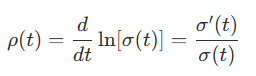
Thus, BDT exhibits mean reversion only if the local volatility term structure is decreasing (σ′(t)<0). If the volatility structure is flat (σ′(t)=0), the BDT model simplifies to the Kalotay-Williams-Fabozzi (KWF) model.

Distribution & Rate Behavior: Because it is a lognormal model, is modeled as r=e^ln(r), meaning interest rates are mathematically restricted from becoming negative. In binomial trees, the possible rates are skewed toward higher rates.

3. The Hull-White (HW) Model

The Hull-White model extends the Ho-Lee model by incorporating explicit mean reversion.

Mathematical SDE: It assumes a normal process for the short rate:

dr = (θ − φr)dt + σdz

where θ is the long-term equilibrium mean rate, and φ is the mean reversion coefficient.

Volatility & Mean Reversion: The mean reversion parameter φ acts as a central tendency, pulling the short rate back toward θ at a specified speed to correct for uncontrolled growth or decline.
Distribution & Rate Behavior: Like Ho-Lee, it is a normal-rate model, meaning negative interest rates are still possible, although the mean reversion parameter significantly reduces their probability. Rates are symmetrically distributed around the mean.
Lattice Implementation: Although it can be mapped to a binomial lattice, the HW model is frequently implemented on a trinomial lattice. The trinomial structure provides three branching paths from each node, offering the mathematical flexibility required to capture mean reversion while maintaining equally spaced time steps.

Structural Impact on Risk Metrics and Valuation

The underlying mathematical assumptions of each model directly dictate the option values, risk metrics, and spreads computed for complex fixed-income securities:

Impact on Option-Adjusted Spread (OAS): Normal models (Ho-Lee and Hull-White) systematically generate higher OAS estimates than lognormal models (KWF, BDT, and Black-Karasinski). Because normal models allow for negative interest rate states, they inflate the expected value of embedded options, which subsequently requires a wider option-adjusted spread to reconcile the model with the security’s observed market price.
Impact on Effective Duration: Lognormal models (such as BDT) yield effective durations that are highly sensitive to prevailing interest rate levels. For example, when interest rates are extremely low, BDT correctly estimates a very short duration for a callable bond, reflecting the high likelihood of an early call. In contrast, normal models (Ho-Lee, Hull-White) produce effective duration estimates that are less sensitive to interest rate levels, sometimes overestimating duration under low-rate extremes.
Impact on Effective Convexity: Lognormal models produce effective convexity patterns that are highly representative of actual pricing behavior. For a callable bond, lognormal trees successfully capture the pricing behavior where effective convexity turns negative (concavity) at intermediate interest rate levels as the embedded call option moves near or into the money.

Lattice Method and Backward Induction

In fixed-income mathematics, an interest rate model mathematically describes how interest rates can change over time. While continuous stochastic differential equations (SDEs) are used to capture interest rate uncertainty, practitioners must convert these continuous equations into discrete, numerical applications to analyze securities. The lattice method serves as the primary tool to achieve this.

1. The Lattice Method (Binomial and Trinomial Lattices)

The lattice method represents future interest rate paths as a discrete grid over time.

Binomial Lattices: In a binomial model, the short-term interest rate can take on only one of two possible values (an up-step or a down-step) at each subsequent node.
Trinomial Lattices: Trinomial models allow for three possible interest rate movements at the next period, offering an extra degree of mathematical freedom.
The Recombining Property: Lattices are typically constructed to recombine, meaning an up-step followed by a down-step results in the identical rate as a down-step followed by an up-step. This recombinatory behavior keeps the tree’s growth linear rather than exponential. Nonrecombining trees grow exponentially (with 2^Nnodes at period N ), making them computationally unwieldy.
Distributional Assumptions: Lognormal trees model interest rates as a lognormal random walk. This restricts the rates in the tree from turning negative, whereas normal interest rate lattices (such as the Ho-Lee model) symmetrically distribute rates around a mean, meaning negative rates are possible.

2. Backward Induction (Recursive Valuation)

Once the lattice is populated with forward interest rates, the arbitrage-free value of a security is calculated using the backward induction (or recursive valuation) methodology.

Working Backward: Under backward induction, the analyst starts at the bond’s maturity (where the terminal payoff of par value plus the final coupon is known with certainty) and works backward from right to left (from the final year in the tree to today).
Valuation at a Node: The value of a bond at any given node depends on its potential future values in the next period. The cash flows one period forward are defined as:
1. The coupon payment (C) plus the bond’s value if the higher forward rate is realized (V_H +C).
2. The coupon payment (C) plus the bond’s value if the lower forward rate is realized (V_L+C).
The Valuation Formula: To find the current node’s value, the present values of these two future cash flows are discounted using the short-term rate (r∗) at the current node. Because the up and down states are assumed to occur with equal probability (50% each), the average of the two present values is taken. The mathematical formula is:

3. Calibration and the No-Arbitrage Constraint

An interest rate lattice is only useful for pricing once it has been calibrated to match the current market term structure.

The Arbitrage-Free Calibration: The rates in the lattice are selected iteratively (using trial-and-error search algorithms) so that the tree’s model-derived prices for option-free benchmark bonds match their actual market prices exactly.
Mathematical Equivalence: Once a tree is calibrated, it is mathematically arbitrage-free and will price an option-free bond identically to the spot curve discounting method.

4. Valuing Embedded Options and Complex Floaters

Lattices and backward induction are highly effective for valuing bonds with embedded options because their future cash flows are interest-rate dependent. As interest rates change across the tree, the likelihood of an option being exercised changes. Lattices incorporate this by adjusting the cash flows at individual nodes:

Callable Bonds: At any node where a bond is eligible to be called, the issuer will call the bond if the present value of future cash flows exceeds the call price. In the tree, the calculated value is replaced by the lesser of the calculated value and the call price.
Putable Bonds: The investor will put the bond if the present value falls below the put price. The value at that node is replaced by the greater of the calculated value and the put price.
Complex Floaters: This recursive node-by-node adjustment also allows the lattice method to price complex floaters—such as range notes (where coupons are paid only if rates fall within a specific band), step-up callable notes, capped floaters, and callable capped floaters.
Option-Adjusted Spread (OAS): Lattices enable the calculation of the OAS—the constant spread that, when added to every forward rate in the interest rate tree, equates the model’s theoretical price to the observed market price.

5. Lattices vs. Monte Carlo: Path-Independence

The critical boundary of the lattice method is that backward induction requires interest-rate-path independence.

Path-Independence: Lattices assume that how the interest rate evolved to get to a specific node does not affect the cash flows at that node. This makes the lattice method highly suitable for corporate, municipal, and sovereign bonds with embedded options.
Path-Dependence: For securities where cash flows are highly path-dependent—such as mortgage-backed securities (MBS) where homeowner prepayment behavior exhibits “burnout” (prepayment incentive depends on the historical path of rates)—the lattice method fails because there is no memory at a node of how rates arrived there. In these instances, Monte Carlo simulation must be used to model cash flows and present values along simulated paths.

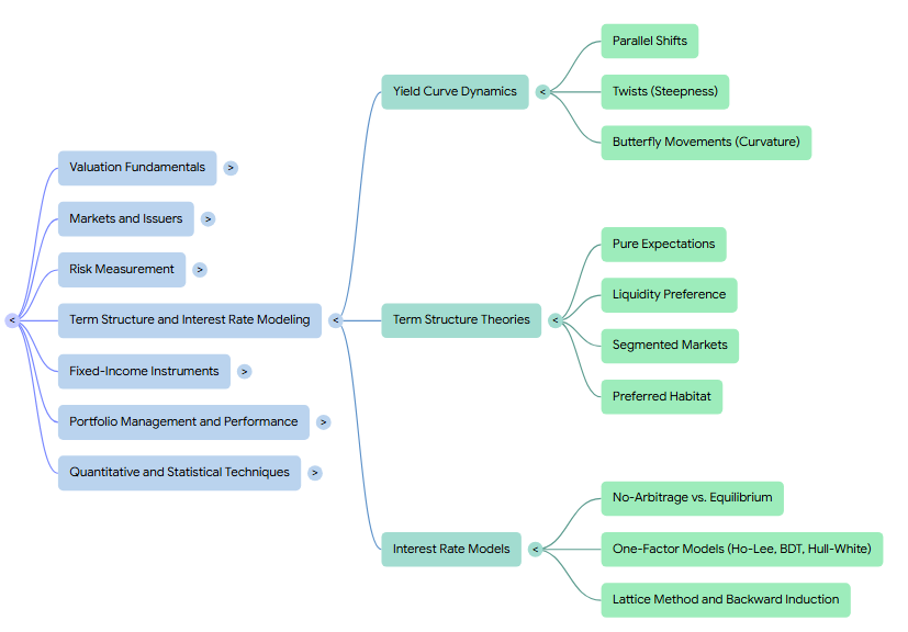
— Linden Lake

This series:
→　Topic Review (1 of 7): Fixed Income – Valuation Fundamentals
→　Topic Review (2 of 7): Fixed Income – Markets and Issuers
→　Topic Review (3 of 7): Fixed Income – Risk Measurement
→　Topic Review (4 of 7): Fixed Income – Term Structure and Interest Rate Modeling
→　Topic Review (5 of 7): Fixed Income – Fixed-Income Instruments
→　Topic Review (6 of 7): Fixed Income – Portfolio Management and Performance
→　Topic Review (7 of 7): Fixed Income – Quantitative and Statistical Techniques

References:
Reference 1, Reference 2, Reference 3

Topic Review (4 of 7): Fixed Income – Term Structure and Interest Rate Modeling

Yield Curve Dynamics

Parallel Shifts

Twists (Steepness)

Butterfly Movements (Curvature)

Term Structure Theories

Pure Expectations

Liquidity Preference

Segmented Markets

Preferred Habitat

Interest Rate Models

No-Arbitrage vs. Equilibrium

One-Factor Models (Ho-Lee, BDT, Hull-White)

Lattice Method and Backward Induction

Leave a Reply Cancel reply