
The time value of money (TVM) serves as the absolute financial foundation for analyzing real estate investments and mortgage structures. Because real estate is inherently a long-term asset and is typically financed with substantial amounts of borrowed capital relative to its purchase price, financing costs play an exceptionally heavy role in the decision to buy property. Under these conditions, the mathematics of TVM are indispensable for calculating mortgage payments, evaluating the true costs of borrowing, and projecting future investment yields.
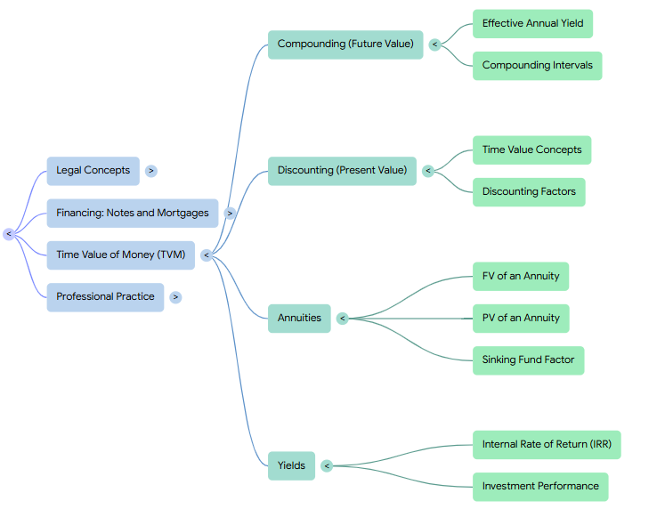
According to the book, the application of TVM to real estate operates through several core pillars:
1. The Mechanics of Compounding (Future Value)
Compounding is the mathematical process of determining what a specific sum of money invested today will grow to over a designated time period at a given interest rate.
- Interest on Interest: The critical engine of compounding is the concept of earning interest on previously accumulated interest, which forms the cornerstone of all financial tables and projections.
- Compounding Intervals: While contracts and mortgage notes in the United States customarily quote a nominal annual interest rate, mortgages utilize monthly compounding almost exclusively.
- Effective Yields: Because compounding frequently occurs monthly rather than annually, the effective annual yield (or annual percentage yield) is higher than the nominal rate. For example, a loan quoted at a nominal annual rate of 12 percent compounded monthly actually carries an effective annual rate of 12.6825 percent compounded annually.
2. The Mechanics of Discounting (Present Value)
Discounting is the exact mathematical inverse of compounding. It is established on the fundamental premise that money has time value; receiving a dollar today is always preferable to receiving a dollar in the future because today’s dollar can be immediately invested to earn interest.
- Cornerstone of Valuation: Discounting adjusts future cash flows back to the present. In real estate, this process is the mandatory starting point for calculating standard mortgage payments, assessing the actual cost of a loan, and determining the market value of income-producing properties.
- The Five Variables: In practice, both compounding and discounting rely on the mathematical interplay of five key variables: the present value (PV), the future value (FV), the interest rate (i ), the number of periods (n), and the periodic payments (PMT).
3. Annuities and Sinking Funds in Real Estate
Most real estate cash flows—whether they are monthly residential mortgage payments, commercial rent receipts, or construction draws—are structured as annuities, which are defined as a series of equal payments or deposits made at equal time intervals.
- Ordinary Annuities vs. Annuities Due: If payments are made at the end of each period (such as standard mortgage payments), they are classified as an ordinary annuity. If payments occur at the beginning of each period, they represent an annuity due.
- Sinking Funds: By dividing a desired future sum by a compounding annuity factor, investors utilize a sinking-fund factor (SFF) to determine the exact monthly or annual payments required to accumulate a specific amount of capital (such as a balloon payment) at a future date.
4. Measuring Investment Performance: Yield and IRR
When investors know the current cost of a real estate asset and can project its future cash flows but do not know the compound rate of return they will earn, they use TVM to calculate the investment yield or internal rate of return (IRR).
- Integrating PV and FV: The IRR fully integrates compounding and present value to identify the single compound rate of interest earned on an outstanding investment balance over the entire holding period.
- Comparing Opportunities: Because real estate transactions can feature highly irregular or uneven cash flow receipts, calculating the IRR is highly beneficial. It translates complex, mismatched cash flow patterns into a single standardized percentage, allowing investors and lenders to easily compare competing projects while fully accounting for the time value of money.
Compounding (Future Value)
At the root of the time value of money (TVM) is the elementary relationship of compound interest. As explained in the book, any compounding problem is constructed from four basic components:
- An initial deposit, representing the present value (PV) of an investment.
- An interest rate (i).
- Time ( n periods or years).
- The value at some specified future period (FV).
1. The Core Mechanic: Interest on Interest
For a single period, the future value is simply the present value plus the interest earned ()during that period:
When extending the timeline to multiple periods, the compounding process continues by treating the ending balance of the first period as the beginning deposit of the second period. Crucially, this means that in subsequent periods, interest is earned not only on the original deposit, but also on the interest accumulated in previous periods. This concept of earning “interest on interest” is the fundamental cornerstone of all financial tables and concepts in financial mathematics.
To find the future value of a single deposit compounded annually for any number of years (), the book details the general formula:
2. Compounding Intervals and Real Estate Mortgages
While basic compounding is framed annually, many financial instruments—such as savings accounts, bonds, and mortgages—compound semiannually, quarterly, monthly, or daily. The book highlights that mortgage loans in the United States involve monthly compounding almost exclusively, making alternative compounding intervals highly important in real estate finance.
To adjust the general compounding formula for other intervals, the nominal annual interest rate () is divided by the number of compounding intervals in a year (), and the total number of periods is scaled to x :
The Impact on Effective Annual Yield (EAY)
Because more frequent compounding allows interest to be earned on interest much sooner, a more frequent compounding interval always yields a higher effective annual yield (EAY) for the same nominal annual interest rate.
To illustrate this “interest on interest” velocity, the book compares the EAY of a 6% nominal annual interest rate across different compounding frequencies:
- Annually (m=1): 6.00%
- Semiannually (m=2): 6.09%
- Quarterly (m=4): 6.14%
- Monthly (m=12): 6.17%
- Daily (m=365): 6.18%
Because nominal interest rates are traditionally quoted in mortgage notes and contracts, real estate professionals must calculate the EAY—which conceptually aligns with the Annual Percentage Yield (APY)—to establish accurate yields and make valid comparisons.
3. Streamlining the Mathematics: Future Value Factors
Historically, performing multi-period compounding calculations manually was incredibly tedious. To solve these problems efficiently, the book explains how compound interest factors were calculated and compiled into tables.
These future value interest factors represent the compounding growth of $1 for various interest rates and time horizons. By identifying the correct factor (using the nominal rate and compounding interval) and multiplying it by the initial present value, investors can easily calculate the future value of any sum. While modern financial calculators and spreadsheet functions (like Excel’s FV function) have largely automated the intermediate step of calculating these factors, the underlying mathematics remain identical.
Effective Annual Yield
In compounding (future value), interest is earned not only on the original principal but also on any accumulated interest from prior periods. While contracts and financial instruments typically quote a nominal annual interest rate as a standard, the book emphasizes that this rate does not represent the actual financial return or cost unless interest is compounded only once per year. To determine the true yield or cost of an investment under different compounding frequencies, we must calculate the Effective Annual Yield (EAY).
What is Effective Annual Yield (EAY)?
The EAY represents the rate of interest actually earned or paid over a one-year period, factoring in the compounding interval. To compute EAY, the book outlines a basic scenario where a principal sum is deposited at the beginning of the year and all proceeds are withdrawn at the end of the year:
For example, if you deposit $10,000 at a nominal annual rate of 6 percent:
- Annual Compounding: The future value (FV) is $10,600, yielding an EAY of 6.00%.
- Monthly Compounding: The is $10,616.78, yielding an EAY of 6.1678%.
This comparison demonstrates that even though the nominal rate (6%) is identical in both cases, the EAY is higher under monthly compounding because interest is computed on ending monthly balances rather than once at the end of the year.
The Impact of Compounding Frequency on EAY
A foundational rule established in the book states that whenever the nominal annual interest rates of two investments are equal, the one with the more frequent compounding interval will always result in a higher EAY.
To illustrate this “interest on interest” velocity, the book compares the EAY of a 6% nominal annual rate across various intervals:
- Annually (m=1): 6.00% EAY
- Semiannually (m=2): 6.09% EAY
- Quarterly (m=4): 6.14% EAY
- Monthly (m=12): 6.17% EAY
- Daily (m=365): 6.18% EAY (or 6.1831% more precisely)
Because of this variance, the book cautions that the nominal interest rate should never be used to compare two investment alternatives with different compounding intervals. Instead, EAY must be computed to form a valid, standardized basis for comparison.
EAY versus Annual Percentage Yield (APY)
The book notes that EAY is conceptually identical to the Annual Percentage Yield (APY) disclosed by banks and savings institutions on financial products like CDs. However, in practice, federal regulations may require banks to include certain fees and penalties in their APY disclosures, which can make the stated APY deviate from the calculated EAY.
EAY in Reverse: Equivalent Nominal Annual Rate (ENAR)
If an investor already has a target EAY and wishes to calculate the matching nominal interest rate for a more frequent compounding interval, they can calculate the Equivalent Nominal Annual Rate (ENAR):
For instance, to match an investment providing an EAY of 6.00%, a competing investment that compounds monthly must offer a nominal annual rate of at least 5.84106%.
Compounding Intervals
Building directly on our previous discussions of the time value of money (TVM) and Effective Annual Yield (EAY), the book details how compounding intervals fundamentally dictate the growth rate of an investment and the true cost of debt.
While the basic formula for compounding (future value) assumes interest is calculated once per year, most real-world investments and debts—such as savings accounts, bonds, and especially U.S. mortgage loans (which use monthly compounding almost exclusively)—operate on shorter compounding intervals.
The Modified Compounding Formula
To account for compounding intervals other than annual, the book explains that the general compound interest formula must be modified. The annual nominal interest rate () is divided by the number of compounding intervals in a year (), and the number of compounding periods is increased by multiplying the years () by :
For example, if an initial deposit of $10,000 earns a nominal annual rate of 6 percent:
- Compounded Annually (m=1): At the end of one year, the future value is $10,600.00.
- Compounded Monthly (m=12): The future value is calculated as , which accumulates to $10,616.78.
The $16.78 difference illustrates the mathematical velocity of “interest on interest”, where interest is calculated and added to the principal balance twelve times a year instead of just once at the end of the year.
The Compounding Interval Rule and Effective Yield
Because more frequent compounding intervals allow interest to be earned on previously accumulated interest much sooner, the book establishes a cardinal rule: whenever the nominal annual interest rates of two investments are equal, the investment with the more frequent compounding interval within the year will always result in a higher effective annual yield (EAY).
To demonstrate this relationship, the book compares the EAY of a 6 percent nominal annual interest rate across varying compounding intervals:
- Annually (m=1): 6.00% EAY
- Semiannually (m=2): 6.09% EAY
- Quarterly (m=4): 6.14% EAY
- Monthly (m=12): 6.17% EAY (specifically 6.1678%)
- Daily (m=365): 6.18% EAY (specifically 6.1831%)
Financial and Investment Comparison Implications
Because contracts, savings accounts, and mortgage notes in the United States customarily quote a nominal annual interest rate and specify the compounding interval in the agreement, understanding the frequency of the interval is critical.
the book cautions that the nominal interest rate should never be used as the basis for comparing two investment alternatives with different compounding intervals. Because of the discrepancy between nominal quotes and actual wealth accumulation, investors must convert the nominal rates to their respective effective annual yields using the interval to establish a standardized, accurate basis for comparison.
Discounting (Present Value)
Within the larger context of the Time Value of Money (TVM), the book describes discounting as the exact mathematical inverse of compounding. While compounding projects a present sum into the future to find its future value, discounting does the opposite: it adjusts future cash receipts back to the present day.
Because real estate is inherently a long-term asset that is heavily financed with loans repaid over time, understanding the present value of future cash flows is vital. Discounting serves as the primary analytical cornerstone for calculating mortgage payments, determining the true cost of loans, and establishing the market value of income-producing properties.
1. The Core Philosophy: Why Money Has Time Value
The concept of present value is built on the fundamental premise that money has time value. If an investor is offered the choice between receiving $1 today or $1 in the future, the correct financial choice is always to accept the $1 today. This is because today’s dollar can be immediately invested to earn interest, making it worth more than a dollar received later.
Consequently, when evaluating future real estate cash flows—whether they are loan payments, rental income, or resale proceeds—investors must apply a “reverse compounding” discount rate to reflect this opportunity cost. The present value represents the maximum amount an investor should pay today to secure those future cash flows while still earning their desired rate of return.
2. Discounting a Single Future Payment (Reversion)
To discount a single lump sum to be received in the future (such as a property’s future resale price, or reversion), the book explains that the general compounding formula is rearranged to solve for the present value (PV):
In this formula, FV is the future value, is the annual interest (or discount) rate, and is the number of years.
- The Reciprocal Relationship: The term () is the present value interest factor (PVIF), which is simply the mathematical reciprocal of the compounding factor .
- Compounding Intervals: Just as compounding can occur at different frequencies, discounting must be adjusted for shorter intervals. Because U.S. mortgage loans almost exclusively use monthly compounding, discounting in real estate is typically calculated using monthly intervals:
This formula divides the annual nominal discount rate by 12 and increases the exponent to reflect the total number of months.
3. Present Value of an Annuity (PVA)
Many real estate cash flows do not occur as single lump sums; instead, they are structured as annuities—a series of equal payments or deposits made at equal time intervals (such as monthly rent or monthly mortgage payments). The book distinguishes between an ordinary annuity (where payments occur at the end of each period) and an annuity due (where payments occur at the beginning of each period).
To find the present value of an ordinary annuity, each individual payment (PMT) must be discounted back to the present day based on the specific period in which it is received, and the results are summed:
Because manually discounting dozens or hundreds of individual periodic payments is highly tedious, the book notes that investors utilize present value of an annuity (PVA) interest factors. Since the periodic payments are constant, the individual discounting factors can be mathematically summed into a single multiplier. For a monthly annuity, this is expressed as:
4. Primary Applications in Real Estate Finance
In the broader real estate market, discounting is applied to make critical investment and financing decisions:
- Valuing Income-Producing Properties: Using discounted cash flow (DCF) techniques, an appraiser or investor determines a property’s current value by discounting the expected annual net operating incomes (NOI) over a holding period, plus the present value of the expected future resale (reversion) price.
- Effective Borrowing Costs: When lenders charge upfront loan fees, origination points, or prepayment penalties, the borrower receives less cash than the nominal loan amount but is still obligated to make payments based on the full face value. By discounting the actual scheduled payments against the net funds disbursed, borrowers can calculate their true effective borrowing cost.
- Lease Comparisons: Landlords and tenants use discounting to calculate the effective net rent of different lease structures (e.g., flat rents, step-up leases, or leases with expense stops and tenant concessions) to reduce complex, varying lease terms into a single, comparable present-value metric.
Time Value Concepts
In the book, time value of money (TVM) concepts are presented as the essential mathematical foundation for analyzing mortgages and real estate investments. Because real estate represents a long-term asset and transactions typically involve significant borrowing repaid over multi-year horizons, mastering these concepts is critical to financial decision-making. Within this broader framework, discounting (present value) serves as the analytical mechanism to adjust future cash receipts back to the present day.
The Core Philosophy of Present Value
The foundation of discounting is the concept that money has time value. The book explains that if an investor is given the choice of receiving $1 today or $1 in the future, the correct financial choice is always to receive it today. This preference exists because today’s dollar can be immediately invested to earn interest, making it inherently worth more than a dollar received down the road.
When determining the price that should be paid today for an asset that is expected to generate future cash flows, investors must apply an adjustment called discounting. This process determines the present value, representing the maximum amount an investor should pay today to achieve their required rate of return.
Discounting as “Reverse Compounding”
The book details that discounting is the exact mathematical inverse of compounding. While compounding projects a present sum into the future, discounting does the opposite by looking backward from a future sum to the present.
- Discounting Single Receipts (Reversions): To discount a single lump-sum receipt to be received in the future (such as the resale price of a property), the future value is multiplied by a present value interest factor (PVIF). This factor is simply the mathematical reciprocal of the compounding interest factor, expressed as:
In real estate, because mortgage loans and investments almost exclusively utilize monthly compounding, this formula is modified to divide the annual interest rate by 12 and multiply the periods by 12 to reflect monthly discounting intervals.
- Present Value of an Annuity (PVA): Real estate cash flows are frequently structured as annuities—a series of equal deposits or payments received at equal time intervals (such as monthly rent or mortgage payments). To find the present value of an annuity, the individual present values of all future payments are summed. The book highlights the distinction between an ordinary annuity, where cash flows occur at the end of each period, and an annuity due, where they occur at the beginning of each period [107n4].
Indispensable Real Estate Applications
The book establishes that present value and discounting concepts are indispensable tools that serve as the cornerstone for several critical applications in real estate finance:
- Calculating Mortgage Payments: Present value mathematics are used to determine the constant periodic payments required to fully or partially amortize a loan over its term.
- Determining True Borrowing Costs: By discounting actual cash receipts against net funds disbursed (after taking into account origination fees and points), borrowers can establish their true effective borrowing cost.
- Appraising Income-Producing Properties: Under the income approach to valuation, appraisers utilize discounted cash flow (DCF) techniques to estimate a property’s market value by discounting its projected net operating income (NOI) and future reversion value back to the present.
- Measuring Investment Yields (IRR): Present value is directly tied to calculating the internal rate of return (IRR), which is the specific discount rate that equates the present value of all expected future cash inflows to the initial investment outlay (resulting in a net present value of zero).
Discounting Factors
Discounting factors—frequently referred to as present value interest factors (PVIF)—are mathematical tools used to determine how much should be paid today for an investment that is expected to produce cash income in the future. Within the larger context of discounting (present value), these factors act as the “reverse” of compounding. They enable investors to translate future cash flows back into present-day dollars, effectively “removing” the compound interest that would otherwise accumulate over time.
1. Mathematical Origin and Single-Payment Factors
In present value analysis, the discounting process is the exact mathematical reciprocal of compounding. According to the book, the discounting factor for a single future payment (often called a reversion) is calculated using the formula:
where is the discount (interest) rate and is the number of periods.
- The Reciprocal Mechanism: To find the present value of a future cash receipt, the future value is multiplied by this reciprocal factor. This calculation establishes the maximum price an investor should pay today to achieve their required rate of return on that investment.
- Compounding and Discounting Intervals: While basic discounting is conceptually framed annually, real estate transactions (such as mortgage loans) utilize monthly discounting intervals almost exclusively. In these cases, the book notes that the discounting factor is modified by dividing the annual interest rate by 12 and multiplying the periods by 12:
Pre-calculated values for these single-payment factors under varying interest rates and periods are compiled in financial tables for both annual reversions (such as Exhibit 3-6) and monthly reversions (such as Exhibit 3-7).
2. Present Value of an Annuity (PVA) Factors
When real estate investments yield an annuity—a series of equal cash payments at equal intervals—the present value can theoretically be found by individually discounting and summing each periodic payment. However, because this manual process is highly tedious, the book explains that the constant nature of the payments allows investors to sum the individual period discounting factors into a single, combined multiplier:
Multiplying the constant periodic payment by this summed Present Value of an Annuity (PVA) factor yields the present value of the entire cash stream in a single step. These cumulative factors are compiled in specialized tables for both annual annuities (Exhibit 3-11) and monthly ordinary annuities (Exhibit 3-12).
3. Practical Utility in the Calculator and Spreadsheet Era
With the advent of financial calculators and spreadsheet software (like Excel), the intermediate step of calculating or looking up discounting factors in tables is often bypassed, as these devices compute the final present value directly.
Nonetheless, the book emphasizes that understanding and utilizing discounting factors remains highly important for two reasons:
- Pedagogical Understanding: Illustrating interest factors allows readers to see and comprehend the actual financial mathematics occurring behind pre-programmed calculator and software solutions.
- Step-by-Step Problem Solving: For complex, multi-part real estate transactions with uneven or grouped cash flows, knowing how to work with these factors allows investors to break down the problem and calculate solutions in manageable steps.
Annuities
Within the larger framework of the time value of money (TVM), the book defines an annuity as a series of equal deposits or payments made at equal time intervals. Because real estate finance primarily deals with long-term assets and liabilities that generate or require steady streams of cash over time—such as monthly mortgage payments, rental receipts, or capital reserve deposits—the mathematical application of annuities is a cornerstone of the discipline.
1. Ordinary Annuities vs. Annuities Due
In financial calculations, the book distinguishes between two primary types of annuities based on the exact timing of the cash flows:
- Ordinary Annuity: This structure assumes that all payments or deposits occur at the end of each designated period [100n3, 101n4]. Most standard real estate contracts, mortgage amortization schedules, and investment valuations operate as ordinary annuities [83, 100n3].
- Annuity Due: This structure assumes that payments or deposits are made at the beginning of each period [101n4]. Real estate leases, where rent is typically due on the first day of the month, are a common example of an annuity due.
2. Future Value of an Annuity (Compounding)
The future value of an annuity represents the cumulative sum of all periodic payments plus the compound interest earned on those deposits over a specified time horizon.
- The Compounding Mechanic: Because payments are constant and occur at equal intervals, each individual deposit compounds for a progressively shorter period of time. For instance, the final payment in an ordinary annuity earns no interest because it is deposited at the exact end of the term [100n3, 101].
- Annuity Factors: To simplify the highly tedious task of compounding each payment individually, the book explains that the constant nature of the payments allows investors to sum individual compounding interest factors into a single Future Value of an Annuity Factor.
- Frequency Adjustments: While basic formulas are often framed annually, the book notes that mortgage payments and investment accounts in the United States operate almost exclusively on monthly schedules. To calculate a monthly compounded annuity, the nominal annual interest rate is simply divided by 12, and the compounding periods are multiplied by 12.
3. Present Value of an Annuity (Discounting)
Evaluating income-producing real estate typically requires looking backward from a series of future cash receipts to determine how much should be paid for an investment today. The present value of an annuity is the sum of the individual present values of all future payments, with each payment discounted back to the present day based on the specific period in which it is received.
- PVA Interest Factors: Rather than discounting dozens or hundreds of individual cash flows, investors utilize compiled tables of Present Value of an Ordinary Annuity Factors. This factor represents the sum of the individual discounting factors for a given interest rate and term.
- Core Applications: Present value annuity math is indispensable in real estate finance. It is the exact mathematical mechanism used to calculate constant monthly mortgage payments, establish the present value of leased fee estates, and determine the effective borrowing cost of a loan.
4. Sinking Funds: Accumulating a Target Future Sum
Frequently, real estate investors or corporate borrowers must establish a systematic savings plan to accumulate a specific lump sum at a future date—such as a capital reserve for property improvements or a balloon payment to retire a mortgage.
To solve for the required periodic deposit, the book utilizes the sinking-fund factor (SFF). The sinking-fund factor is the mathematical reciprocal of the future value of an annuity factor. Multiplying a target future sum by the sinking-fund factor yields the exact constant payment that must be deposited each period to reach the financial goal, factoring in the compound interest those deposits will earn.
5. Yields and the Internal Rate of Return (IRR) on Annuities
When the initial purchase price (present value) and the future stream of equal cash receipts (annuity) of an investment are known, TVM concepts allow investors to calculate the investment yield or internal rate of return (IRR).
The IRR on an annuity is the specific compound rate of interest that equates the present value of all expected future cash inflows to the initial investment outlay. Under a level annuity structure, the book demonstrates that each periodic payment received by the investor implicitly contains two distinct financial components: the recovery of capital (principal return) and the interest earned on the outstanding, unrecovered investment balance.
FV of an Annuity
In the book, an annuity is defined as a series of equal payments or deposits made at equal time intervals. Within the larger context of financial mathematics, the Future Value (FV) of an annuity represents the cumulative sum of these periodic payments plus all compound interest earned on them over a specified time horizon.
Ordinary Annuities vs. Annuities Due
The mathematical calculation of an annuity’s future value is heavily dictated by the exact timing of the cash flows:
- Ordinary Annuity: This structure assumes that all payments or deposits occur at the end of each period [103n3, 104n4]. Most standard real estate contracts and mortgage structures operate as ordinary annuities. Because of this timing, each deposit is compounded for a progressively shorter period. Crucially, the final deposit does not earn interest because it occurs at the exact end of the final year [103n3, 104].
- Annuity Due: This structure assumes that deposits or payments are made at the beginning of each period [104n4]. Real estate leases, where rent is traditionally due on the first of the month, are a classic example of an annuity due.
The Mathematics of Accumulation and Interest Factors
To calculate the future value of an ordinary annuity, the individual compounded values of each periodic payment (P) must be mathematically summed. For an annual compounding schedule, the expanded formula is:
To simplify this highly tedious task, the book explains that when the periodic payments are constant, the individual compounding interest factors can be summed into a single Future Value of an Annuity Factor. Multiplying the constant periodic payment by this cumulative factor yields the total future value in a single, efficient step.
Adjusting for Monthly Compounding
While basic models are often framed annually, the book notes that real estate finance and investment accounts in the United States operate almost exclusively on monthly schedules. To adjust the future value formula for monthly compounding, the nominal annual interest rate () is divided by 12, and the compounding periods are scaled to months ():
The Broader Real Estate Context: Sinking Funds
In the broader context of real estate finance, calculating the future value of an annuity is essential for planning future cash requirements. A primary application of this concept is the sinking fund, which is a systematic savings plan used to accumulate a targeted lump sum at a future date—such as to fund major property capital improvements or pay off a balloon mortgage balance. To determine the constant payment required to reach a future goal, the target sum is multiplied by the sinking-fund factor (SFF). The sinking-fund factor is the mathematical reciprocal of the future value of an annuity factor, demonstrating how closely the accumulation of future real estate wealth is structurally tied to the compounding mechanics of annuities.
PV of an Annuity
In the book, the Present Value (PV) of an annuity is defined as the sum of the individual present values of a series of equal, periodic cash flows (receipts or payments) discounted back to the present day. While the future value of an annuity focuses on the accumulation of wealth over time, the present value of an annuity focuses on valuation—specifically, determining how much a buyer or investor should pay today to secure a series of future cash receipts at a required rate of return.
In the larger context of annuities, the present value concept is a foundational pillar of real estate finance, serving as the mathematical underlayment for property valuation, mortgage amortization, lease comparisons, and yield calculations.
1. The Mathematical Framework of Discounting an Annuity
An annuity consists of equal payments (or receipts) made at equal intervals. The book primarily focuses on an ordinary annuity, which assumes that all cash flows occur at the end of each period [90n3, 102].
To find the present value of an ordinary annuity, each individual payment (PMT) must be discounted back to the present day based on the specific period in which it is received, and these discounted values are then summed:
In this formula, is the discount (required) rate, and is the number of periods. Because the first payment is not received until the end of the first period, it is discounted for only one period (); the second payment is discounted for two periods, and so on, until the final payment is discounted for periods.
2. Streamlining with Present Value of an Annuity Factors
Discounting dozens or hundreds of individual periodic cash flows manually is highly tedious and inefficient. The book explains that because the payments in an annuity are constant, the individual present value discounting factors can be mathematically summed into a single, combined multiplier, known as the Present Value of an Ordinary Annuity Factor:
- Annual Annuities: For annual cash flows, the summed interest factors for varying interest rates and years are compiled in the book under Exhibit 3-11. For example, an investment that returns $500 per year for six years at a required return of 6% has a cumulative annuity factor of 4.917324. Multiplying $500 by this factor yields a present value of $2,458.66.
- Monthly Annuities: Because standard real estate transactions—such as mortgage payments and rental cash flows—occur monthly, the compounding and discounting interval is typically adjusted to monthly periods. The formula divides the annual nominal interest rate () by 12 and multiplies the years () by 12. These cumulative monthly ordinary annuity factors are compiled in the book under Exhibit 3-12. For instance, a monthly annuity of $500 for 12 months discounted at a nominal annual rate of 6% compounded monthly uses a factor of 11.618932, resulting in a present value of $5,809.47.
3. Indispensable Applications in Real Estate Finance
In the book, the present value of an annuity is applied dynamically across several key financing and investment areas:
- Mortgage Loan Amortization: A mortgage loan is structurally the present value of an annuity. When a lender provides a fully amortizing, constant payment mortgage (CPM), the loan amount represents the present value, and the borrower’s scheduled monthly payments represent the annuity. For example, for a $60,000 loan made at a 12% interest rate for 30 years (360 months), solving for the constant monthly payment (PMT) required to fully amortize the loan yields $617.17.
- Property Valuation (Discounted Cash Flow Analysis): Under the income capitalization approach, investors utilize discounted cash flow (DCF) techniques. The value of an income-producing property is estimated by taking the present value of its annual net operating incomes (NOIs), which often resemble a step-up or indexed annuity, and adding it to the present value of the future resale price (reversion). In the Oakwood Apartments case study, the present value of the projected NOIs over a five-year holding period at an 11% discount rate is $3,694,762, which is added to the present value of the resale proceeds ($6,879,172) to estimate the total property value at $10,573,934.
- Effective Rent and Lease Comparisons: Leases can have highly complex structures involving stepped-up rents, expense stops, moving allowances, or free rent. To make an “apples-to-apples” comparison between competing lease proposals, the book explains that managers calculate the present value of the expected net rental streams. They then divide this total present value by the ordinary annuity factor over the lease term to calculate the effective net rent—which represents the equivalent level annuity of those cash flows.
Sinking Fund Factor
Continuing our discussion on the time value of money (TVM) and annuities, the book introduces the sinking-fund factor (SFF) as a crucial mathematical concept for accumulating a future target sum. While our previous discussions focused on finding the future value (accumulation) or present value (valuation) of a known annuity stream, the sinking fund calculation does the reverse: it determines the size of the periodic payments (the annuity) required to accumulate a predetermined future lump sum.
1. Mathematical Reciprocal of the Future Value of an Annuity
Under the compounding framework, finding the future value of an ordinary annuity involves multiplying a series of equal payments by a cumulative Future Value of an Annuity (FVA) factor. When trying to find the required payment to meet a future target, we must mathematically isolate the periodic payment (PMT).
the book demonstrates that this is done by dividing the target future value by the FVA interest factor:
Dividing a number by the FVA factor is mathematically identical to multiplying it by the factor’s reciprocal:
This reciprocal, (), is defined in real estate finance as the sinking-fund factor (SFF).
To illustrate, the book presents a scenario where a borrower must repay a $20,000 debt in one lump sum at the end of five years. Assuming the deposits can earn a 10 percent annual interest rate, the corresponding annual FVA factor is 6.105100. Isolating the payment can be done in two equivalent ways:
- Division Method: Dividing the $20,000 target by 6.105100 yields an annual payment of $3,275.95.
- Multiplication Method (SFF): The reciprocal of the FVA factor is 1/6.105100=0.163797, which represents the sinking-fund factor. Multiplying the target sum of $20,000 by this SFF (0.163797) yields the exact same annual payment of $3,275.95.
This calculation shows that making five annual payments of $3,275.95 at the end of each year will successfully accumulate $20,000 by the end of year five, with the help of compound interest.
2. Compounding Frequency Adjustments
In real estate finance, transactions and interest accruals rarely happen on a strictly annual basis; most follow monthly schedules. the book notes that the sinking-fund calculation can easily be adjusted for monthly compounding by dividing the nominal annual interest rate by 12 and multiplying the years by 12 to find the total number of monthly periods.
Using the same $20,000 debt scenario over five years (60 months) with an annual interest rate of 10 percent compounded monthly (i=10%/12=0.833%), the monthly payment is computed using these adjusted variables:
- Monthly Sinking Fund Payment: Solving for the payment yields required monthly deposits of $258.27.
3. Practical Applications in Real Estate Finance
In the broader real estate market, the sinking-fund factor is an indispensable tool with several key applications:
- Lump-Sum Debt Retirement: It allows corporate borrowers and property owners to structure regular, equal contributions to accumulate the necessary funds to completely retire balloon mortgages or other lump-sum liabilities coming due at a future date.
- Capital Replacement Reserves (CAPEX): Property managers and investors use the SFF to calculate the periodic reserves that must be set aside to fund non-recurring, long-term capital improvements. For example, if a roof must be replaced in 10 years at an estimated cost of $100,000, the owner can use the SFF to determine the exact monthly cash reserves that must be deducted from operations to build that future fund, factoring in the compound interest those reserves will earn over the decade.
Yields
In the larger context of the Time Value of Money (TVM), the book presents the determination of yields—also referred to as the internal rate of return (IRR)—as the ultimate tool for measuring and comparing investment performance over time. The book draws a conceptual distinction between “interest rates” and “yields,” noting that the term interest rate is typically utilized when lenders quote nominal loan terms, whereas yield or IRR is preferred when evaluating the actual compound rate of return earned on an outstanding investment [120n6, 122].
According to the TVM framework laid out in the book, yields are analyzed and determined through several core applications:
1. Yields on Investments with Single Receipts
When an investment involves a single cash outlay in the present (present value, or PV) and is held to receive a single cash return in the future (future value, or FV), the yield represents the compound interest rate that equates the two. Using the fundamental TVM present value formula:
the book demonstrates that we must solve for the unknown rate . This calculated yield integrates the concepts of compounding and present value, representing the equivalent annual compound rate of interest earned over the entire holding period.
2. Yields on Investment Annuities
When an investment produces a series of equal, periodic cash receipts over time (an annuity), calculating the yield is more complex because the cash flows are spread out across multiple periods. The book highlights that the calculated yield (IRR) on an annuity represents a rate of compound interest earned on the outstanding, unrecovered investment balance after accounting for periodic capital recovery.
Implicitly, each periodic annuity payment contains two distinct financial components:
- The recovery of a portion of the initial capital (principal return).
- The interest or profit earned on the outstanding, unrecovered investment balance during that period.
3. Yield Adjustments: Effective Annual Yield (EAY) and ENAR
A critical TVM principle established in the book is that nominal interest rates should not be used to compare different investment options unless their compounding intervals are identical. To standardize comparisons, investors must calculate the Effective Annual Yield (EAY), which measures the actual rate earned over a one-year period by factoring in the frequency of compounding:
- The Compounding Interval Rule: If nominal rates are equal, the investment with the more frequent compounding interval (e.g., monthly vs. annually) will always yield a higher EAY because interest is calculated and added to the principal balance sooner.
- Equivalent Nominal Annual Rate (ENAR): If an investor has a target EAY but is evaluating an alternative that compounds more frequently (such as monthly), they can use the ENAR formula to determine the minimum nominal rate required to match that target EAY.
4. Yields with Partial Periods and Irregular Cash Flows (XIRR)
When an investment is sold prematurely (such as mid-year) or generates irregular, uneven cash flows, traditional compounding and annuity formulas become inadequate. To resolve this, the book introduces the XIRR (Extended Internal Rate of Return) method. By assigning exact calendar dates to each cash flow, the XIRR formula discounts each receipt based on the fraction of the year (days/365) to find the precise discount rate that brings the net present value of the investment to zero.
Internal Rate of Return (IRR)
In the book, “yield” and “internal rate of return” (IRR) are often used interchangeably when evaluating the performance of real estate investments, while the term “interest rate” is typically reserved for quoting loan terms. Both concepts conceptually represent the compound rate of interest earned on an investment. However, within the broader context of yields, the internal rate of return (IRR) provides a highly sophisticated, standardized metric to analyze and compare real estate opportunities under varying conditions.
1. The Core Mechanic of IRR
The IRR is mathematically defined as the discount rate (or compound rate of interest) that equates the present value of all expected future cash flows over a specified holding period to the initial investment outlay, resulting in a net present value (NPV) of zero.
While simple yields are easy to solve for single-receipt investments or level annuities, real estate cash flows are frequently irregular and vary from period to period. In these more complex scenarios, solving for the IRR requires an iterative “trial and error” process to find the precise discount rate that brings the present value of those mismatched cash flows in line with the initial equity investment.
2. Capital Recovery vs. Compound Interest
The book emphasizes that when the IRR is calculated on a real estate investment, the return implicitly contains two distinct financial components:
- The recovery of capital (the return of the initial principal).
- The interest or profit earned on the outstanding, unrecovered investment balance during each period.
Thus, the IRR does not simply measure total cash received; it measures the compound rate of interest earned on the outstanding capital actively tied up in the property from year to year.
3. Leveraged vs. Unleveraged and Tax-Adjusted Yields
To dynamically analyze investment performance, the book breaks the IRR down into several classifications depending on financing and tax structures:
- Unleveraged IRR: The total compound return generated by the property asset itself, calculated as if the investor paid all cash and used no debt financing.
- Before-Tax Leveraged IRR (BTIRR): The return earned on the investor’s actual equity contribution after debt service is deducted from the operating cash flows. If the unleveraged IRR exceeds the cost of debt, the BTIRR will be magnified, resulting in positive financial leverage.
- After-Tax IRR (ATIRR): The ultimate measure of net yield, which incorporates federal income tax liabilities, capital gains taxes, and the benefits of non-cash depreciation tax shelters.
4. Partitioning the IRR for Risk Assessment
Because a high projected yield can often mask underlying investment risk, the book highlights partitioning the IRR as a vital risk-assessment tool. This technique splits the total present value of the investment’s cash flows into its two primary components:
- The proportion of the return derived from annual operating cash flows.
- The proportion of the return derived from the sale of the property (reversion) at the end of the holding period.
If a dominant portion of the IRR is heavily weighted toward future price appreciation and resale proceeds (reversion), the yield is considered highly sensitive to future market changes and therefore carries significantly greater risk than an investment whose yield is supported primarily by stable, ongoing tenant lease payments.
5. IRR (Dollar-Weighted) vs. Time-Weighted Returns (TWR)
In institutional portfolio management, the book notes that the IRR is also referred to as a dollar-weighted return because it is heavily influenced by the exact volume and timing of cash flows into and out of a fund. When evaluating fund managers, the choice between utilizing IRR or a time-weighted return (TWR) depends entirely on control:
- Use IRR when the investment manager has direct control over the timing and volume of capital calls and property sales (typically in closed-end value-added or opportunistic funds).
- Use TWR when the manager has no control over when investors choose to contribute or redeem capital (typically in open-end core funds where investors enter and exit at will). The TWR eliminates the distorting effect of these external capital flows, allowing for an “apples-to-apples” comparison of management skill.
Investment Performance
In the book, investment performance is analyzed as a multi-dimensional concept that cannot be evaluated by nominal yields alone. Portfolio managers must continually measure real estate yields—derived from periodic cash flows and capital appreciation—to compare them dynamically against other asset classes like common stocks, corporate bonds, and government securities.
To build a rigorous performance framework, the book details specific metrics to calculate yields, adjust for risk, evaluate portfolio-level benefits, and isolate manager-specific value.
1. Yield Metrics for Measuring Return Performance
To quantify investment performance, the book outlines several key mathematical yields:
- Holding Period Return (HPR): This represents the fundamental, single-period unit of investment performance, calculating the sum of price changes and dividends relative to the beginning price.
- Arithmetic vs. Geometric Mean: When analyzing a series of returns over time, the book notes a key conceptual difference. The arithmetic mean is a simple, non-compounded average. Conversely, the geometric mean (or time-weighted return) represents the true compounded rate of return over the entire investment horizon and is considered superior for evaluating past performance because it is not distorted by periodic volatility.
- TWR (Time-Weighted Return) vs. IRR (Internal Rate of Return):
- Time-Weighted Return (TWR): This chain-links individual HPRs, giving equal weight to each period’s return regardless of the volume of capital invested. It is the optimal measure when a fund manager does not have control over capital inflows and outflows (such as open-end commingled core funds where investors can enter and exit at will).
- Internal Rate of Return (IRR / Dollar-Weighted): This measures the compound rate of return on the outstanding capital actively tied up in the investment. It is heavily influenced by the exact timing and dollar magnitude of cash flows. This is the preferred metric when a fund manager has direct control over the timing of capital calls and distributions (such as closed-end, value-added, or opportunistic funds).
2. Public vs. Private Real Estate Performance Data
A major challenge highlighted in the book is the discrepancy between the performance data available for public versus private real estate:
- Public Real Estate (NAREIT Equity Index): Based on the share prices of publicly traded Equity REITs, this index represents real estate operating on a leveraged basis. Because shares trade in continuous auction markets, REIT returns are highly liquid but take on the volatility of the public stock market, exhibiting a high correlation with the S&P 500.
- Private Real Estate (NCREIF Property Index): Based on individual properties held by pension funds, this index is computed on an unleveraged, “free and clear” basis. Because properties trade in thin, negotiated markets, NCREIF relies heavily on quarterly appraisals. Appraisals tend to lag behind sudden market shifts, which creates a “smoothing effect” that artificially lowers the index’s reported standard deviation. However, NCREIF exhibits a stronger correlation with the CPI, proving to be a highly effective historical inflation hedge.
3. Integrating Risk: Risk-Adjusted Return Metrics
Because higher returns are typically accompanied by higher price volatility, the book emphasizes that nominal yields must be adjusted to measure true performance. Key risk-adjusted benchmarks include:
- Coefficient of Variation: Calculated as the standard deviation of returns divided by the mean return, measuring the amount of risk taken per unit of return. By this measure, private real estate (NCREIF) historically outperforms leveraged public real estate (REITs) on a risk-adjusted basis due to its lower appraisal-induced volatility.
- The Sharpe Ratio: Standardizes excess performance by dividing the fund’s average return over the risk-free rate by the standard deviation of its returns.
- The Treynor Ratio: Similar to Sharpe, but divides excess returns by beta (systematic risk) to measure how much excess return is delivered per unit of market-correlated risk.
- Tracking Error & Information Ratio: Tracking error measures the standard deviation of the difference in returns between a fund and its benchmark. The Information Ratio divides the average excess return by the tracking error to evaluate whether a manager’s outperformance is a consistent behavior.
- Jensen’s Alpha: Measures whether an active manager generated excess returns (value-added “alpha”) above what would be expected under the Capital Asset Pricing Model (CAPM) given the fund’s systematic risk (beta).
4. Portfolio Performance and the Efficient Frontier
Under modern portfolio theory, the performance of an individual asset should not be judged in isolation, but rather by how it impacts the risk and return of an entire portfolio.
- Diversification Benefits: When assets with low or negative correlation coefficients (less than +1) are combined, the standard deviation of the portfolio’s return is reduced without necessarily sacrificing the average return.
- The Efficient Frontier: This represents the optimal combination of assets providing the maximum expected return for a given level of risk. The book demonstrates that incorporating real estate (both public and private) into a traditional stock-and-bond portfolio shifts the efficient frontier upward, allowing institutional investors to capture higher portfolio yields at lower overall risk thresholds.
5. Decomposing Performance: Attribution Analysis
To evaluate whether an active fund manager has successfully achieved a target yield, the book utilizes attribution analysis to break down performance relative to a benchmark. This isolates two key manager functions:
- Selection Effect: Value added by the manager’s ability to select superior individual properties within a specific sector or region compared to the benchmark.
- Allocation Effect: Value added by successfully over-weighting sectors or regions that outperform the overall benchmark, or under-weighting lagging sectors.
By calculating these effects mathematically, investors can determine if a manager’s outperformance was driven by skillful asset curation, macro-allocation strategy, or simply taking on uncompensated risk.
— Linden Lake
This series:
→ Book Review (1 of 4): Real Estate Finance and Investments – Legal Concepts
→ Book Review (2 of 4): Real Estate Finance and Investments – Financing: Notes and Mortgages
→ Book Review (3 of 4): Real Estate Finance and Investments – Time Value of Money(TVM)
→ Book Review (4 of 4): Real Estate Finance and Investments – Professional Practice
Leave a Reply