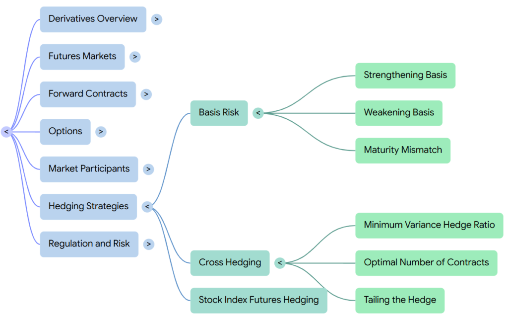
Book Review (6 of 7): Options, Futures, and Other Derivatives – Hedging Strategies

In the book, hedging strategies are presented as fundamental risk-management tools utilized by corporations, financial institutions, and portfolio managers to neutralize or insure against exposures to volatile market variables. Rather than seeking to generate speculative profits, the core objective of a hedger is risk reduction by stabilizing future cash flows and minimizing the variance of a portfolio’s value.

1. The Core Philosophy of Hedging

A central tenet emphasized in the book is that hedging is designed to reduce risk, not to maximize profits. There is no guarantee that a company will achieve a better financial outcome with a hedge than without one.

The Symmetrical Trade-off: If the market moves in an adverse direction, the hedge provides vital protection. However, if the market moves in a favorable direction, the company will perform worse than if it had remained unhedged because the gains on the physical business are offset by losses on the derivative contracts.
Why Companies Choose Not to Hedge: Despite the clear benefits of risk reduction, many corporate exposures are left unhedged. Shareholders can often diversify risks more cheaply on their own, making firm-level hedging redundant under some financial theories. Furthermore, if competitors in an industry do not hedge, a single company that hedges may actually increase the volatility of its profit margins relative to the industry standard. Corporate treasurers also face the “treasurer’s dilemma,” where they are criticized for losses incurred on derivatives hedges even when those losses are fully offset by gains in the physical business.

2. Linear Hedging: Forwards and Futures

Forwards and futures are used to completely lock in a price, thereby neutralizing the risk of subsequent price fluctuations.

Short Hedges: Appropriate when a company already owns an asset (or expects to own it) and plans to sell it in the future. For example, an oil producer can short crude oil futures to lock in a selling price for its future production, guaranteeing a fixed revenue regardless of how low spot prices fall.
Long Hedges: Appropriate when a company knows it must purchase an asset in the future and wants to lock in a price today. A copper fabricator, for instance, can go long copper futures to stabilize its raw material costs and avoid “unpleasant surprises” from rising input prices.
Basis Risk: In practice, a perfect hedge is rare due to basis risk, which is the uncertainty associated with the final “basis” (defined as the spot price of the asset to be hedged minus the futures price of the contract used) at the time the hedge is closed out. A strengthening basis unexpectedly improves a short hedger’s position and worsens a long hedger’s position, while a weakening basis does the opposite.
Cross Hedging and the Minimum Variance Hedge: When the asset being hedged is different from the asset underlying the futures contract, the company must execute a cross hedge. To minimize the variance of the hedged position, the optimal hedge ratio (h∗) must be calculated as:

$h^* = \rho \frac{\sigma_S}{\sigma_F}$

where ρ is the correlation between spot and futures price changes, and σ_S and σ_F are their respective standard deviations.

Stack and Roll: If a company’s hedging horizon exceeds the maturity of liquidly traded contracts, it can employ a stack and roll strategy—buying short-term contracts and rolling them forward into subsequent contracts near expiration. However, this introduces severe liquidity risk, as short-term price drops can force massive cash outflows (margin calls) on the futures positions long before the gains on the physical contracts are realized, a mismatch that led to a $1.33 billion loss for Metallgesellschaft.

3. Asymmetric Hedging: Options and Insurance

Unlike forwards and futures, which obligate both parties to execute a transaction, options provide a form of insurance. They allow hedgers to establish a protective price floor or cap while retaining the ability to benefit from highly favorable market moves, in exchange for an upfront payment called the option premium.

Covered Calls: An investor writes a call option while holding a long position in the underlying stock. The stock position “covers” the short call against unlimited upside risk, and the premium received provides a small buffer against price declines [537, 791 note 3].
Protective Puts: An investor buys a put option on a stock they already own [537, 65 note 1]. This guarantees a minimum selling price (intrinsic strike) for their shares while keeping the upside open if stock prices rise. Under put-call parity, this is equivalent to buying a European call option and holding cash.
Range Forwards: Commonly used in foreign exchange markets, a range forward is a zero-cost contract created by buying a European put option at a lower strike price K1 and selling a European call option at a higher strike price K2. This setup provides a range within which the final exchange rate is realized, offering downside protection in exchange for sacrificing extreme upside potential.

4. Equity Portfolio Hedging and Portfolio Insurance

The book outlines specific strategies used by portfolio managers to manage systematic risk in well-diversified equity portfolios.

Stock Index Futures: A manager can completely hedge or adjust the beta (β) of an equity portfolio by shorting index futures contracts. The optimal number of contracts required is calculated as:

$N^* = \beta \frac{V_A}{V_F}$

where V_A is the current value of the portfolio and V_F is the value of one futures contract. This allows managers who are adept at “stock picking” to eliminate broader market risk and isolate their portfolio’s relative outperformance.

Portfolio Insurance: Managers can buy index put options to establish a floor on the portfolio’s value. This can also be done synthetically without buying actual options by dynamically trading the underlying equities or index futures. To replicate a protective put, the manager must continuously maintain a position in the index or index futures equal to the delta of the required option. This requires selling assets as the market declines and buying them back as it rises. However, during the October 1987 crash, stock exchange systems became so overloaded that portfolio managers could not sell index futures fast enough, proving that synthetic portfolio insurance can fail during extreme market disruptions.

5. Advanced Dynamic Hedging and the “Greeks”

Because option parameters change continuously with asset price movements and the passage of time, standard static hedges are insufficient for derivatives dealers. Dealers must manage their risk dynamically by keeping a suite of sensitivity measures, known as the Greeks, close to zero.

Delta Hedging: Delta (Δ) is the rate of change of the option price with respect to the price of the underlying asset. A dealer maintains delta neutrality (Δ=0) by holding a position of −Δ shares of the underlying asset for each long option held. This hedge must be frequently rebalanced.
Gamma Hedging: Gamma (Γ) measures the curvature of the option price relationship, representing the rate of change of delta. If gamma is large (positive or negative), the delta is highly sensitive to price changes, increasing the risk of hedging errors. A portfolio is made gamma neutral by adding traded options.
Vega Hedging: Vega measures the sensitivity of the portfolio to changes in the asset’s implied volatility. To protect against volatility shifts, dealers add traded options to make the portfolio vega neutral.
Outside Model Hedging: Although pricing models like Black-Scholes-Merton assume volatility is constant, traders still actively calculate vega and hedge against volatility changes in the real world—a process known as hedging outside the model [1270, 1275 note 17].

Basis Risk

In the book, a perfect hedge—one that completely eliminates risk—is noted to be extremely rare. Instead, most real-world hedges are subject to basis risk, which arises due to the uncertainty regarding what the “basis” will be at the time the hedge is closed out.

The basis is formally defined as:

Basis = Spot price of asset to be hedged − Futures price of contract used

If the asset being hedged is identical to the asset underlying the futures contract, the basis will converge to zero at the exact expiration of the futures contract. However, prior to expiration, the basis can be either positive or negative. As time passes, the spot price and the futures price do not necessarily change by the same amount, which causes the basis to fluctuate.

Mathematical Impact on Hedging Outcomes

To analyze this risk, the book utilizes the following parameters for a hedge initiated at time t₁ and closed out at time t₂:

S₁, S₂ : Spot prices at times t₁and t₂.
F₁, F₂ : Futures prices at times t₁ and t₂.
b₁, b₂ : Basis values at times t₁ and t₂ (where b_i = S_i−F_i).

Short Hedges (The Seller’s Perspective)

For a hedger who plans to sell the underlying asset at t₂ and initiates a short futures position at t₁, the effective price realized for the asset is:

Effective Price = S₂+F₁−F₂=F₁+b₂

Since the initial futures price F1 is locked in and known at t1, the entire uncertainty regarding the final price realized is determined by the final basis b2.

Long Hedges (The Buyer’s Perspective)

For a hedger who plans to buy the asset at t₂ and initiates a long futures position at t₁, the effective price paid is:

Effective Price = S₂+F₁−F₂=F₁+b₂

Just as with the short hedge, the final effective price paid is F₁+b₂, making the hedging risk strictly dependent on the uncertainty of the final basis b₂ .

The Dynamics of Basis Movements: Strengthening vs. Weakening

Changes in the basis over the life of a hedge directly impact the financial position of the hedger:

Strengthening of the Basis: Occurs when the basis increases (b₂ > b₁).
- For a short hedge, an unexpected strengthening improves the company’s position because they realize a higher net price for their asset.
- For a long hedge, an unexpected strengthening worsens the company’s position because they pay a higher net price.
Weakening of the Basis: Occurs when the basis decreases (b₂ < b₁).
- For a short hedge, an unexpected weakening worsens the position.
- For a long hedge, an unexpected weakening improves the position.

Real-World Causes of Basis Risk

The book identifies three primary structural complications in hedging strategies that generate basis risk:

Asset Mismatch (Cross Hedging): The asset whose price is being hedged is not exactly the same as the asset underlying the futures contract.
Timing Mismatch: There is uncertainty regarding the exact date when the physical asset will be bought or sold.
Contract Maturity Mismatch: The hedge requires closing out the futures contract prior to its delivery month.

Cross Hedging and Volatility Management

When a cross hedge is necessary (such as an airline using heating oil futures to hedge its exposure to jet fuel), basis risk is significantly increased. In this scenario, the book decomposes the basis into two distinct components:

$\text{Payoff Price} = F_1 + \left(S_2^* – F_2\right) + \left(S_2 – S_2^*\right)$

Where $S_2^*$ is the spot price of the asset underlying the futures contract at t₂. The term $\left(S_2^* – F_2\right)$ is the basis that would exist if there were no asset mismatch, whereas the $\left(S_2-S_2^*\right)$ term represents the additional basis risk arising purely from the difference between the two assets.

To minimize the variance of a cross-hedged position, a hedge ratio of is often suboptimal. Instead, the hedger must calculate and apply the minimum variance hedge ratio (h∗):

$h^* = \rho \frac{\sigma_S}{\sigma_F}$

Where σ_S is the standard deviation of the change in spot price (ΔS ), σ_F is the standard deviation of the change in futures price (ΔF ), and ρ is the correlation coefficient between the two. The optimal number of contracts ( $N^*$ ) to trade is then determined by:

$N^* = \frac{h^* Q_A}{Q_F}$

where Q_A is the size of the position being hedged, and Q_F is the size of one futures contract. When daily settlement is considered, the formula is adjusted to reflect percentage changes rather than absolute changes, and the position can be “tailed” to account for interest earned or paid on daily margin.

Minimizing Basis Risk: Contract Selection

A hedger can actively manage and minimize basis risk by carefully choosing the contract specifications, which involves two decisions:

Choosing the Underlying Asset: The hedger must select the available futures contract whose price is most highly correlated with the asset being hedged.
Choosing the Delivery Month: The book highlights that futures prices can be highly erratic during the delivery month, and long hedgers run the risk of facing expensive and logistically inconvenient physical delivery. Consequently, hedgers normally close out contracts before the delivery month.
The Rule of Thumb: A reliable guideline for hedgers is to choose a delivery month that is as close as possible to, but later than, the expiration of the hedge. This minimizes the time difference between the hedge expiration and the delivery month, which directly reduces the size of the basis risk.

Strengthening Basis

In the book, basis risk is a central complication in hedging, arising from the reality that a perfect hedge—one that completely eliminates risk—is extremely rare. Instead, most real-world hedges face uncertainty because of the basis, which is defined as:

Basis=Spot price of asset to be hedged−Futures price of contract used

This basis changes over time because spot prices and futures prices do not necessarily change by the exact same amount. An increase in the basis is formally termed a strengthening of the basis, while a decrease is referred to as a weakening of the basis.

The Context of Basis Risk

The book notes that basis risk arises primarily from three real-world mismatches:

Asset Mismatch: The physical asset being hedged is not identical to the asset underlying the futures contract (known as cross hedging).
Timing Mismatch: There is uncertainty regarding the exact date when the physical asset will be bought or sold.
Maturity Mismatch: The hedge requires closing out the futures contract prior to its delivery month.

Prior to a contract’s expiration, the basis can be either positive or negative. Because the basis is not constant, a hedger cannot know today exactly what the basis will be when the hedge is closed out. The uncertainty associated with this final basis (b₂) is the core of basis risk.

Impact of a Strengthening Basis on Hedgers

To understand how a strengthening basis impacts a hedge, we look at the final effective price. At the time of close-out (t₂), the net effective price obtained (for a seller) or paid (for a buyer) is mathematically equal to:

Effective Price=F₁+b₂

where F₁ is the initial futures price locked in at the start of the hedge (t₁), and b₂ is the final basis at the close-out of the hedge (t₂). Since F₁ is known at the start, the final net price is entirely dependent on the movement of the final basis b₂ .

For Short Hedgers (Sellers): A short hedge is used when a company plans to sell an asset in the future. If the basis strengthens (increases) unexpectedly, the company’s position improves. This is because a higher basis (b₂) results in a higher net effective price (F₁+b₂) realized for the sold asset after factoring in futures gains or losses.
For Long Hedgers (Buyers): A long hedge is used when a company plans to buy an asset in the future. If the basis strengthens unexpectedly, the company’s position worsens. A higher basis (b₂) means the company must pay a higher net effective price (F₁+b₂) to acquire the asset.

Conversely, a weakening of the basis produces the exact opposite effects—worsening the position of a short hedger but improving the position of a long hedger.

Weakening Basis

In the book, a weakening of the basis is defined as a decrease in the basis over time . The basis itself is the difference between the spot price of the asset being hedged and the futures price of the contract used to construct the hedge :

Basis=Spot price of asset to be hedged−Futures price of contract used

While the basis converges to zero at the exact expiration of a matching futures contract, it can fluctuate and be positive or negative prior to expiration because spot and futures prices do not necessarily change by the same amount .

The Larger Context of Basis Risk

A perfect hedge that completely eliminates risk is rare in practice . Instead, hedgers must manage basis risk, which is the financial uncertainty arising from the fact that the basis at the time the hedge is closed out (the final basis, b₂) is not known today .

According to the book, this risk is typically driven by three real-world complications :

Asset Mismatch (Cross Hedging): The physical asset being hedged is not identical to the asset underlying the futures contract .
Timing Mismatch: There is uncertainty regarding the exact calendar date when the physical asset will be bought or sold .
Maturity Mismatch: The hedge requires the futures contract to be closed out prior to its actual delivery month .

Impact of a Weakening Basis on Hedging Outcomes

To understand how a weakening basis impacts a hedger, the book evaluates the effective price realized at the close-out of the hedge . For both buyers and sellers, this net price is mathematically defined as:

Effective Price = F₁+b₂

where F₁is the initial futures price locked in when the hedge is initiated, and b₂ is the final basis when the hedge is closed out . Because F₁ is a known constant, any change in the final basis directly alters the net price .

For Short Hedgers (Sellers): A short hedge is used by a participant who plans to sell the underlying asset in the future . If the basis weakens (decreases) unexpectedly, the company’s position worsens . This is because a lower final basis (b₂) reduces the net effective price (F₁+b₂) they receive for the physical asset after factoring in their futures gains or losses .
For Long Hedgers (Buyers): A long hedge is used by a participant who knows they must purchase an asset in the future . If the basis weakens unexpectedly, the company’s position improves . The decrease in b₂ lowers the net effective price (F₁+b₂) they must pay to acquire the asset after accounting for the hedge .

Conversely, a strengthening (increase) of the basis has the exact opposite effect—improving the short hedger’s position and worsening the long hedger’s position .

Maturity Mismatch

In the book, a maturity mismatch—specifically the requirement that a futures contract be closed out prior to its delivery month—is identified as one of the three primary causes of basis risk. Along with asset mismatches (which require cross hedging) and uncertainty regarding the exact transaction date, a mismatch in timing or maturity prevents the hedger from achieving a perfect hedge.

1. How Maturity Mismatch Drives Basis Risk

The basis is contractually defined as the difference between the spot price of the asset being hedged and the futures price of the contract used:

Basis=Spot Price−Futures Price

The Convergence Ideal: If the asset being hedged is identical to the asset underlying the futures contract, the basis will converge to exactly zero at the contract’s maturity.
The Mismatch Reality: If a hedger is forced to close out the hedge before the delivery month of the futures contract, the basis will not have converged to zero. Because spot and futures prices do not change by the same amounts over time, this final basis (b₂) is highly uncertain.
The Impact of Distance: The book states that basis risk increases as the time difference between the hedge expiration and the contract’s delivery month increases. Therefore, a wider maturity mismatch directly amplifies the risk that changes in the basis will adversely affect the final net price paid or received.

2. Mitigating Mismatch: The “Close But Later” Rule of Thumb

To actively manage and minimize the basis risk generated by maturity mismatches, the book outlines a standard rule of thumb for contract selection:

The Rule: A hedger should choose a delivery month that is as close as possible to, but later than, the expiration of the hedge.
The Logic: This minimizes the time difference (the maturity mismatch) between the transaction date and the delivery month, thereby keeping the basis risk as small as possible. For example, if a hedge expires in January, and the available delivery months are March, June, September, and December, the March contract is selected because it is the closest available maturity that falls after the hedge’s expiration.

3. The Liquidity Trade-Off and “Stack and Roll” Risks

While matching maturities as closely as possible is theoretically ideal, hedgers must contend with market liquidity:

Liquidity Constraints: In practice, market liquidity is almost always greatest in short-maturity futures contracts.
The Rollover Strategy: If a company has a long-term exposure but long-dated futures contracts lack sufficient liquidity, the hedger may be forced to use short-term contracts and roll them forward sequentially (a stack and roll strategy).
Severe Cash-Flow Risks: Rolling hedges forward introduces an acute form of maturity mismatch. If the spot price moves adversely during the hedge’s life, the company will face immediate, daily cash outflows (margin calls) on its short-term futures positions, while the offsetting gains on the long-term physical assets will not be realized until years later.
Historical Failure: This specific cash-flow mismatch led to the catastrophic collapse of the German company Metallgesellschaft in the early 1990s, which incurred a $1.33 billion loss when severe short-term cash drains forced management to abandon its rolled hedges.

4. Maturity Mismatch in the Broader Banking Context (ALM)

Beyond transactional hedging, the book explores maturity mismatch in the wider context of banking and asset-liability management (ALM).

The Mismatch Dilemma: Banks naturally operate with a maturity mismatch because depositors prefer to put their funds into short-term deposits (for financial flexibility), while borrowers prefer long-term, fixed-rate loans like mortgages (to lock in borrowing costs).
Interest Rate Risk: If interest rates rise, the bank’s short-term funding costs will rise immediately, while its long-term asset yields remain fixed, severely squeezing net interest income.
Liquidity Risk: Beyond interest rate exposure, a severe maturity mismatch exposes a bank to liquidity risk—the danger that short-term wholesale depositors may lose confidence and refuse to roll over funding. Even a well-capitalized bank can be forced into bankruptcy if it cannot fund its long-term assets with short-term liabilities, a dynamic that directly caused major failures during the 2007–2009 financial crisis, including Northern Rock, Bear Stearns, and Lehman Brothers.

Cross Hedging

In the broader context of hedging strategies, cross hedging occurs when the asset whose price is being hedged is different from the asset underlying the futures contract used to construct the hedge. This strategy is a vital tool for corporate risk managers when there is no liquidly traded futures contract that directly matches their physical exposure. For example, the book highlights that because jet fuel futures are not actively traded, an airline will typically use highly liquid heating oil futures to hedge its jet fuel price exposure [184, 194 note 3].

1. The Amplification of Basis Risk

Cross hedging significantly increases basis risk. When direct hedging is used with a matching underlying asset, the basis converges to zero at the futures contract’s expiration. In a cross hedge, however, the mismatch between the two assets ensures that the basis will remain volatile even at contract maturity.

To analyze this risk, the book decomposes the basis at the close-out of a cross hedge into two distinct components:

$\text{Basis} = \left(S_2^* – F_2\right) + \left(S_2 – S_2^*\right)$

$S_2^* – F_2$ represents the basis that would exist if the asset being hedged were identical to the asset underlying the futures contract.
$S_2 – S_2^*$ represents the additional basis risk arising purely from the price discrepancy between the two different assets (e.g., the price difference between jet fuel and heating oil at time ).

2. The Suboptimality of a 1.0 Hedge Ratio

The hedge ratio is the ratio of the size of the position taken in futures contracts to the size of the physical exposure. While it is natural to use a hedge ratio of 1.0 when the underlying assets match, doing so in a cross hedge is rarely optimal. Instead, the corporate treasurer must select a specific hedge ratio that minimizes the variance of the value of the hedged position.

3. Calculating the Minimum Variance Hedge Ratio ( $h^*$ )

By modeling the relationship between the change in the spot price (ΔS) and the change in the futures price (ΔF ) as approximately linear, the book derives the minimum variance hedge ratio ( $h^*$ ):

$h^* = \rho \frac{\sigma_S}{\sigma_F}$

where:

σ_S is the standard deviation of ΔS,
σ_F is the standard deviation of ΔF, and
ρ is the correlation coefficient between the two price changes.

These parameters are typically estimated using historical data (such as weekly or monthly price changes), under the implicit assumption that the future price behavior will mirror the past.

Hedge Effectiveness

The effectiveness of the cross hedge—defined as the proportion of the variance eliminated by the hedge—is represented by the R² value from the regression of ΔS against ΔF, which mathematically equals ρ².

4. The Optimal Number of Contracts ( $N^*$ )

Once the minimum variance hedge ratio $h^*$ is determined, the optimal number of futures contracts ( $N^*$ ) required to construct the hedge is calculated as:

$N^* = \frac{h^* Q_A}{Q_F}$

where Q_A is the total size of the physical position being hedged, and Q_F is the standardized size of a single futures contract.

5. Adjustments for Daily Settlement and Tailing

Because futures contracts are settled daily rather than at the end of their life, a static hedge can experience minor daily drift. To account for this, the book outlines two refinements:

The Percentage Change Model: Instead of regressing absolute price changes, managers can regress daily percentage changes in spot prices against daily percentage changes in futures prices to derive an alternative hedge ratio, $\hat{h} = \hat{\rho}\frac{\hat{\sigma}_S}{\hat{\sigma}_F}$ . The number of contracts then adjusts to $N^* = \frac{\hat{h}V_A}{V_F}$ , where V_A is the current dollar value of the physical portfolio (SQ_A) and V_F is the current dollar value of one futures contract (FQ_F ).
Tailing the Hedge: To incorporate the interest earned or paid on daily margin balances over the remaining life of the hedge, the optimal number of contracts can be “tailed” by dividing $N^*$ by 1+r (where r is the risk-free rate of interest over the hedge’s remaining life).

Minimum Variance Hedge Ratio

In the book, cross hedging occurs when the physical asset whose price is being hedged is different from the asset underlying the futures contract used to construct the hedge. Because the underlying instruments do not match, cross hedging inherently increases the basis risk of the position.

When the underlying assets match, it is standard to use a hedge ratio of 1.0. However, in a cross-hedging scenario, using a 1.0 ratio is rarely optimal. Instead, the corporate treasurer must select a specific hedge ratio that minimizes the variance of the overall value of the hedged position. This optimal ratio is known as the minimum variance hedge ratio ( $h^*$ ).

1. Mathematical Derivation of $h^*$

To determine this ratio when daily settlement is ignored, the book models the relationship between the change in the spot price (ΔS ) and the change in the futures price (ΔF ) over the life of the hedge as approximately linear:

ΔS = a + bΔF + ϵ

where a and b are constants and ϵ is an error term.

If a percentage h of the spot exposure is hedged using futures, the change in the value of the combined position per unit of exposure is:

ΔS − hΔF = a + (b−h)ΔF + ϵ

The standard deviation (and thus the variance) of this hedged position is minimized when the second term on the right-hand side is eliminated. This occurs when we set the hedge ratio h equal to b .

Using the standard formula for the slope of a linear regression, the minimum variance hedge ratio ( $h^*$ ) is defined as:

$h^* = \rho \frac{\sigma_S}{\sigma_F}$

where:

σ_S is the standard deviation of ΔS.
σ_F is the standard deviation of ΔF.
ρ is the correlation coefficient between ΔS and ΔF.

If the futures price moves in perfect lockstep with the spot price ( ρ=1 and σ_S = σ_F ), the optimal hedge ratio is exactly 1.0 . If the futures price is twice as volatile as the spot price but remains perfectly correlated ( ρ=1 and σ_F = 2σ_S ), the optimal ratio is 0.5 .

2. Hedge Effectiveness and Parameter Estimation

The proportion of the variance that is eliminated by executing the minimum variance hedge represents the hedge effectiveness. This is mathematically equivalent to the R² coefficient from the regression of ΔS against ΔF, which is equal to ρ² .

In practice, the parameters ρ, σ_S, and σ_F are estimated using historical data, assuming that past price relationships will continue to hold in the future. The data is gathered over several equal, nonoverlapping time intervals. Ideally, the length of these historical intervals should match the planned duration of the hedge, though shorter intervals are frequently used if available data is limited.

3. Calculating the Optimal Number of Contracts ( $N^*$ )

To implement the hedge, the optimal number of futures contracts ( $N^*$ ) is calculated by applying the minimum variance hedge ratio to the total physical exposure:

$N^* = \frac{h^* Q_A}{Q_F}$

where Q_A represents the total size of the position being hedged (in units of the physical asset) and Q_F represents the standardized size of a single futures contract.

As an example, the book describes an airline that plans to purchase 2 million gallons of jet fuel in one month (Q_A=2,000,000) and decides to cross hedge its exposure using heating oil futures contracts, which are traded more actively [104, 105 note 3]. Based on historical monthly data, the standard deviations are σF=0.0313 and σS=0.0263, with a correlation of ρ=0.928.

The minimum variance hedge ratio is calculated as:

$h^* = 0.928 \times \frac{0.0263}{0.0313} = 0.78$

Since each heating oil contract represents 42,000 gallons (Q_F = 42,000):

$N^* = \frac{0.78 \times 2{,}000{,}000}{42{,}000} \approx 37.14\ \text{contracts}$

Rounding to the nearest integer, the airline should short 37 heating oil contracts.

4. Incorporating Daily Settlement (Tailing the Hedge)

Because exchange-traded futures are settled daily, they effectively act as a series of sequential one-day hedges rather than a single static transaction. The book notes that we can adjust for this by regressing daily percentage changes (returns) rather than absolute price changes.

If $\hat{\sigma}_S$ is the daily standard deviation of percentage changes in the spot price, $\hat{\sigma}_F$ is the daily standard deviation of percentage changes in the futures price, and $\hat{\rho}$ is their daily correlation, the adjusted hedge ratio ( $\hat{h}$ ) is:

$\hat{h} = \hat{\rho}\frac{\hat{\sigma}_S}{\hat{\sigma}_F}$

Under this framework, the optimal number of contracts to trade is:

$N^* = \frac{\hat{h}V_A}{V_F}$

where V_A is the total monetary value of the physical asset being hedged (V_A=SQ_A ) and V_F is the monetary value of a single futures contract (V_F = FQ_F ). This hedge ratio is dynamic and liable to adjust slightly over time as spot and futures prices fluctuate.

Finally, this calculation can be refined by tailing the hedge. Tailing accounts for the interest that is earned or paid on the daily variation margin flows over the remaining life of the hedge. To tail the hedge, the computed number of contracts ( $N^*$ ) is divided by 1 + r, where r is the applicable risk-free interest rate over the hedge’s remaining life.

Optimal Number of Contracts

In the book, the optimal number of contracts (denoted as $N^*$ ) is the precise quantity of futures contracts required to construct a hedge that minimizes the overall variance of the hedged position. In a cross hedge—where the asset being hedged differs from the asset underlying the futures contract—simply matching the exposure on a 1.0 basis is rarely optimal because the prices of the two assets do not move in perfect lockstep.

The Standard Formula (Without Daily Settlement)

To calculate the optimal number of contracts under a static “hedge-and-forget” strategy, the corporate treasurer must apply the minimum variance hedge ratio ( $h^*$ ). The formula for the optimal number of contracts is:

$N^* = \frac{h^* Q_A}{Q_F}$

where:

Q_A is the total size of the physical position being hedged (measured in units).
Q_F is the standardized size of a single futures contract.
$h^*$ is the minimum variance hedge ratio, calculated as $h^* = \rho \frac{\sigma_S}{\sigma_F}$ .

For example, the book illustrates this with an airline hedging the purchase of 2 million gallons of jet fuel (Q_A = 2,000,000) using heating oil futures contracts, where each contract represents 42,000 gallons (Q_F=42,000). With an estimated hedge ratio of $h^*$ =0.78 derived from historical price data, the optimal number of contracts is:

$N^* = \frac{0.78 \times 2{,}000{,}000}{42{,}000} \approx 37.14\ \text{contracts}$

Rounding to the nearest whole number, the airline should short 37 contracts.

Adjustments for Daily Settlement (Marking to Market)

In practice, exchange-traded futures contracts are settled daily rather than at the end of their life, which effectively turns the hedge into a series of sequential one-day hedges. To account for this daily settlement, the book details an alternative approach that works with daily percentage price changes (returns) instead of absolute price changes:

1. Percentage-Based Hedge Ratio ( $\hat{h}$ ): A percentage-based hedge ratio is calculated as:

$\hat{h} = \hat{\rho}\frac{\hat{\sigma}_S}{\hat{\sigma}_F}$

where $\hat{\sigma}_S$ is the daily standard deviation of percentage changes in the spot price, $\hat{\sigma}_F$ is the daily standard deviation of percentage changes in the futures price, and $\hat{\rho}$ is their correlation.

2. Adjusted Contract Formula: Under this percentage change framework, the optimal number of contracts is:

$N^* = \frac{\hat{h}V_A}{V_F}$

where V_A=SQ_Ais the total monetary value of the physical position being hedged and V_F =FQ_F is the current monetary value of a single futures contract (the futures price multiplied by the contract size).

Because spot and futures prices fluctuate daily, the optimal number of contracts is dynamic and liable to adjust slightly from day to day. However, these daily shifts are usually small and frequently ignored by traders in practice.

Refining for the Time Value of Money: Tailing the Hedge

To achieve even greater precision, the calculated number of contracts can be adjusted to account for the interest earned or paid on the cash flows generated by daily margin changes over the remaining life of the hedge. This process is known as tailing the hedge. To tail the hedge, the raw contract number is $N^*$ divided by 1 + r (where r is the risk-free rate of interest over the hedge’s remaining life).

Tailing the Hedge

In the book, tailing the hedge is presented as an essential refinement used to adjust the optimal number of futures contracts to account for the time value of money over the life of a hedge.

To understand its role, it must be viewed in the larger context of cross hedging and the unique daily cash flows of futures contracts.

1. The Cross Hedging Foundation

When a company must hedge a risk but no liquid futures contract exists for its exact underlying asset, it must perform a cross hedge using a related asset (such as an airline using heating oil futures to hedge jet fuel). Because the price of the hedging instrument does not move in perfect lockstep with the asset being hedged, the company cannot simply use a standard 1.0 hedge ratio.

Instead, the treasurer calculates a minimum variance hedge ratio ( $\hat{h}$ or $h^*$ ) based on the historical correlation and volatility of the two assets. This ratio is then used to calculate the optimal number of contracts ( $N^*$ ) required to minimize the portfolio’s overall variance:

Under a standard model, the raw number of contracts is determined by $N^* = \frac{h^* Q_A}{Q_F}$ .
When accounting for daily settlement, the formula can be expressed in terms of the monetary value of the exposure (V_A ) and the value of one futures contract (V_F ), yielding $N^* = \frac{\hat{h}V_A}{V_F}$ .

2. The Impact of Daily Settlement

A basic, unadjusted hedging model is theoretically appropriate for forward contracts because forwards are settled as a single lump-sum cash flow at the end of their maturity. Futures contracts, however, are subject to daily settlement (marking to market).

At the end of each trading day, the margin account is adjusted to reflect the day’s gains or losses, causing cash (variation margin) to flow daily between the long and short positions. Consequently, a futures contract behaves like a series of consecutive one-day hedges rather than a single static hedge.

Because of these daily cash flows, the hedger either earns interest on positive margin balances or must pay interest to finance margin calls over the remaining life of the hedge.

3. Adjusting for the Time Value of Money: Tailing the Hedge

To neutralize the interest rate impact of these daily margin cash flows, the hedger must perform the tailing procedure. Tailing the hedge involves discounting the raw optimal number of contracts ( $N^*$ ) to reflect the interest that will be earned or paid over the remaining life of the hedge.

Mathematically, this refinement is executed by dividing the optimal number of contracts ( $N^*$ ) by (1 + r) , where r is the risk-free interest rate per annum over the hedge’s remaining life:

For example, if the applicable risk-free interest rate is 5% per annum and the hedge has a remaining life of one year, the analyst must divide $N^*$ by 1.05 to arrive at the tailed contract amount.

By reducing the initial number of contracts today, the hedger prevents the interest compounding on daily margin cash flows from over-hedging or under-hedging the physical position by the time the contract matures.

Stock Index Futures Hedging

In the book, stock index futures hedging is presented as a highly effective tool for managing, adjusting, or entirely neutralizing the systematic risk of a well-diversified equity portfolio. In the broader context of hedging strategies—which typically focus on static “hedge-and-forget” risk-reduction positions—hedging with stock index futures utilizes the portfolio’s systematic market sensitivity to stabilize returns.

The Underlying Asset and Cash Settlement

A stock index tracks the performance of a hypothetical portfolio of stocks, typically focusing on capital gains and losses because dividends are usually excluded from the index calculation. Because it is logistically inconvenient or impossible to physically deliver the hundreds of stocks comprising an index, the book notes that stock index futures are strictly settled in cash. Upon contract maturity, all outstanding positions are closed out at the spot price of the index on that day.

The Systematic Hedging Formula

When a corporate treasurer or portfolio manager seeks to hedge a well-diversified equity portfolio, the optimal number of futures contracts to trade depends directly on the portfolio’s beta (β).

Beta as the Hedge Ratio: Under capital asset pricing theory, beta represents the portfolio’s sensitivity to market movements. Mathematically, the book shows that using beta as the scaling factor is equivalent to the percentage-based hedge ratio ( $\hat{h}$ ) calculated in commodity cross-hedging.

The Optimal Number of Contracts ( $N^*$ ): If a portfolio perfectly mirrors the index (β=1.0), the number of contracts to short is simply the portfolio value divided by the futures contract value ( $N^* = \frac{V_A}{V_F}$ ). When the portfolio’s beta is not 1.0, the formula generalizes to:

$N^* = \beta \frac{V_A}{V_F}$

where V_A is the current value of the stock portfolio and V_F is the current value of a single futures contract (the futures price multiplied by the contract size).

Growth at the Risk-Free Rate

A complete hedge (reducing the portfolio’s beta to zero) removes all systematic market risk. In accordance with financial theory, once market risk is neutralized, the combined position (the long stock portfolio plus the short index futures) is expected to grow at the risk-free interest rate.

To demonstrate this, the book provides a detailed numerical example of a $5,050,000 portfolio with a beta of 1.5, hedged by shorting 30 futures contracts. Whether the stock index rises or falls over a three-month period, the gain or loss on the short futures position offsets the expected CAPM-based return of the stock portfolio, ensuring that the total value of the hedger’s position remains stabilized and grows at the risk-free rate of 4% per annum (or 1% over the three months).

Strategic Motivations for Hedging vs. Liquidating

It is natural to wonder why an investor should execute a futures hedge to earn the risk-free rate rather than simply selling their stocks and purchasing risk-free bonds. The book outlines two primary justifications for index futures hedging:

Locking in the Benefits of “Stock Picking”: If a portfolio manager believes they possess a unique ability to select undervalued stocks that will outperform the market, they can short $\beta \frac{V_A}{V_F}$ index futures contracts. This removes the broad market’s systematic return, leaving the manager exposed solely to the relative outperformance of their stock selections. If their chosen stocks perform better than the market index (after adjusting for beta), the manager will lock in a profit regardless of whether the overall market goes up or down.
Avoiding High Transaction Costs: An investor may expect highly volatile, negative market conditions in the short term but wish to maintain their stock holdings for the long term. Rather than liquidating the portfolio and repurchasing it later—which would incur unacceptably high transaction and commission costs—the investor can temporarily short stock index futures to achieve cheap, short-term protection.

Adjusting Portfolio Beta

Beyond complete immunization (targeting a beta of zero), index futures hedging can be applied dynamically to adjust a portfolio’s beta to any other desired level. For instance, if a manager expects a market downturn but does not want to exit the market entirely, they can short a partial amount of index futures to temporarily reduce their portfolio’s beta from 1.5 to 0.5. This flexibility allows managers to dial their market exposure up or down rapidly without buying or selling the underlying physical shares.

— Linden Lake

This series:
→　Book Review (1 of 7): Options, Futures, and Other Derivatives – Derivative Overview
→　Book Review (2 of 7): Options, Futures, and Other Derivatives – Futures Markets
→　Book Review (3 of 7): Options, Futures, and Other Derivatives – Forward Contracts
→　Book Review (4 of 7): Options, Futures, and Other Derivatives – Options
→　Book Review (5 of 7): Options, Futures, and Other Derivatives – Market Participants
→　Book Review (6 of 7): Options, Futures, and Other Derivatives – Hedging Strategies
→　Book Review (7 of 7): Options, Futures, and Other Derivatives – Regulation and Risk

Book Review (6 of 7): Options, Futures, and Other Derivatives – Hedging Strategies

Basis Risk

Strengthening Basis

Weakening Basis

Maturity Mismatch

Cross Hedging

Minimum Variance Hedge Ratio

Optimal Number of Contracts

Tailing the Hedge

Stock Index Futures Hedging

Leave a Reply Cancel reply