Book Review (2 of 5): Valuation – Core valuation Techniques

In the book, Part Two, “Core Valuation Techniques,” is designed as a self-contained handbook that translates the fundamental economic principles of value creation into a rigorous, step-by-step mathematical methodology. While the foundations of value establish that Return on Invested Capital (ROIC) and growth drive free cash flows, core valuation techniques provide managers and investors with the practical tools to measure, analyze, and manage that value.

In the larger context of corporate valuation, the book organizes these core techniques into a highly structured, sequential workflow.

1. Valuation Frameworks (Chapter 10)

The book details several discounted cash flow (DCF)-based valuation models, demonstrating that when applied with consistent assumptions, they yield identical results:

Enterprise Discounted Cash Flow (DCF) Model: This is the primary model used by practitioners and academics. It discounts projected Free Cash Flow (FCF)—the cash flow available to all investors, independent of capital structure—at the Weighted Average Cost of Capital (WACC). Equity value is then calculated indirectly by subtracting debt and other nonequity claims from the resulting enterprise value.
Discounted Economic Profit Model: This model defines Economic Profit as the spread between ROIC and WACC, multiplied by the invested capital: The operating value of a company equals its book value of invested capital plus the present value of all future economic profits. While mathematically equivalent to the enterprise DCF model, this framework provides deeper strategic insights by explicitly highlighting when and where a company is actually creating or destroying value on a year-by-year basis.
Adjusted Present Value (APV) Model: APV separates the value of operations into two components: the value of operations as if the company were entirely equity-financed and the value of interest tax shields arising from debt financing. It is the most flexible model when a company’s capital structure is expected to change significantly (such as in a leveraged buyout or debt pay-down schedule) [403, 446, 478n1].
Cash-Flow-to-Equity (CFE) Model: CFE discounts cash flows directly to equity holders at the levered cost of equity. It is highly prone to implementation errors because capital structure changes are embedded directly in the cash flows, but it remains the preferred method for valuing banks and other financial institutions where capital structure is an inextricable part of daily operations.

2. The Reorganization of Financial Statements (Chapter 11)

Traditional financial statements commingle operating performance and financing structures, making them inadequate for direct economic analysis. The book establishes that reorganizing the financial statements is a crucial first step to isolate the core drivers of value:

Invested Capital: Reorganizing the balance sheet to isolate the actual investor capital required to fund operations, without distinguishing how that capital is financed. This involves calculating operating working capital, property, plant, and equipment (PP&E), and other operating assets net of operating liabilities.
Net Operating Profit After Taxes (NOPAT): Reorganizing the income statement to calculate the after-tax operating profit generated by the company’s invested capital. To calculate NOPAT, only operating costs and depreciation are deducted from revenues, while operating cash taxes are computed on operating profits as if the company held only operating assets and was financed entirely with equity.
Free Cash Flow (FCF): Derived as NOPAT minus the net increase in invested capital, representing the cash flow available to all debt and equity holders.

3. Analyzing Historical Performance (Chapter 12)

Core valuation techniques require a thorough historical analysis (typically looking back at least ten years) to establish a realistic baseline for future projections:

ROIC with and without Goodwill: The book requires analyzing ROIC both including and excluding goodwill. ROIC with goodwill measures the company’s ability to create value over and above the price premiums paid for past acquisitions. ROIC excluding goodwill measures the underlying competitiveness and operating performance of the business, which serves as the proper baseline for forecasting.
Decomposing ROIC: ROIC is broken down into operating margins (profitability) and capital turnover (capital productivity).
Revenue Growth Decomposition: Historical revenue growth must be stripped of distortions—namely, currency fluctuations, mergers and acquisitions (M&A), and accounting policy changes—to identify the true organic revenue growth rate of the business.
Financial Health: Analyzing liquidity and leverage using coverage ratios (such as EBITDA-to-interest) and debt multiples (such as debt-to-EBITDA) to evaluate the sustainability of the capital structure.

4. Forecasting Performance (Chapter 13)

A proper valuation model relies on a forecast of free cash flows generated by projecting the income statement, balance sheet, and statement of equity in an integrated manner:

The Primacy of Revenues: The book emphasizes that the revenue forecast is the most critical component of the model because almost every other line item is directly or indirectly driven by revenues.
Transitioning Detail: Forecasters should project line-by-line financial details in the short term (first few years) to capture near-term operational realities, but transition to high-level value drivers (operating margins, capital efficiency) in the medium term (5 to 15 years).

5. Estimating Continuing Value (Chapter 14)

Since explicitly forecasting cash flows year-by-year into perpetuity is impractical, the book utilizes a continuing value formula to value the cash flows beyond the explicit forecast period.

The Key Value Driver Formula: The book strongly recommends the Key Value Driver Formula over simple cash flow perpetuities:

This formula is superior because it explicitly links continuing value to the rate of return expected on new capital investments (RONIC), capturing the core economic truth that a company must reinvest a portion of NOPAT to grow.

Steady-State Requirement: Continuing value formulas should only be applied once the company has reached a steady state with stable margins, WACC, and growth.

6. Estimating the Cost of Capital (Chapter 15)

The WACC represents the opportunity cost of capital to the company’s investors, blending the expected returns required by equity and debt holders.

Cost of Equity: Estimated via the Capital Asset Pricing Model (CAPM). Because historically measured individual company betas are highly imprecise, the book advises using unlevered industry peer medians to determine operating risk, which are then relevered to the company’s target capital structure.
Cost of Debt: Approximated using the yield to maturity of the company’s long-term, option-free bonds (for investment-grade debt).
Weights: Weighted using forward-looking target market-value weights of debt and equity, rather than book values, which represent irrelevant sunk costs.

7. Moving from Enterprise Value to Value per Share (Chapter 16)

Once the value of operations is calculated, the core valuation process requires a rigorous buildup to convert enterprise value into equity value per share:

Add Nonoperating Assets: Add the market value of assets not captured in free cash flow, including excess cash, investments in nonconsolidated companies, and tax loss carryforwards.
Subtract Nonequity Claims: Subtract all financial claims that have priority over common equity, including interest-bearing debt, debt equivalents (such as capitalized operating leases and unfunded pension/retirement obligations), and hybrid claims (such as convertible debt and outstanding employee options) valued using options-pricing models.
Divide by Undiluted Shares: Divide the residual equity value by the current undiluted shares outstanding (not diluted shares, to avoid double-counting hybrid claims already deducted).

8. Analyzing and Validating the Results (Chapter 17)

The final phase of the core valuation process is putting the completed model to work and testing its robustness:

Technical Robustness: Ensuring the balance sheet balances every year and NOPAT reconciles perfectly with net income.
Economic Consistency: Checking that the projected financial and operating ratios are consistent with competitive dynamics (e.g., ROIC cannot expand indefinitely in a competitive industry without attracting rivals who force margins down).
Plausibility & Multiples Check: Comparing the implied forward-looking valuation multiples of the model (like EV/EBITA or EV/NOPAT) against peer companies to identify and explain discrepancies.
Sensitivity and Scenario Analysis: Developing probability-weighted scenarios to bound and quantify the underlying strategic uncertainties of the future.

9. Core Complementary Tools: Multiples and Valuation by Parts

Using Multiples (Chapter 18): Multiples serve as a vital relative-valuation check against the DCF model. The book strongly advocates using forward-looking net enterprise value to EBITA (or NOPAT) multiples because they are not distorted by different capital structures, nonoperating items, or tax jurisdictions.
Valuation by Parts (Chapter 19): For companies with multiple business segments, top-down valuations are highly inaccurate. Core techniques dictate valuing the company by its parts (sum-of-the-parts), creating separate operating statements and applying segment-specific WACCs and peer multiples to each unit before aggregating.

Valuation Frameworks

In the book, Part Two is designed as a self-contained guide to Core Valuation Techniques, which translates the high-level economic principles of corporate finance into practical, step-by-step methodologies. The absolute foundation of these techniques begins in Chapter 10 with selecting the appropriate Valuation Framework. While there are multiple ways to value a business, the book focuses heavily on discounted cash flow (DCF) and economic profit-based approaches, proving that when applied with consistent assumptions, they yield identical results.

Within the larger context of measuring and managing corporate value, choosing the right framework is crucial because each model carries distinct analytical benefits and implementation risks. The book categorizes and evaluates these frameworks across five primary models:

1. Enterprise Discounted Cash Flow (DCF) Model

The Mechanics: This model discounts projected Free Cash Flows (FCF) at the Weighted Average Cost of Capital (WACC). It determines equity value indirectly by subtracting debt and other nonequity claims from the resulting enterprise value.
Best Application: It is highly favored by academics and practitioners because it relies strictly on the actual cash flowing in and out of the company, independent of capital structure. It works best for projects, business units, and companies that manage their capital structure to a target level.
The Limitation: The book notes that a major shortfall of enterprise DCF is that a single year’s FCF provides very little insight into a company’s competitive position or economic health. For example, a healthy company that is investing heavily in its future will show depressed near-term FCF, making it superficially look like a poor performer.

2. Discounted Economic Profit Model

The Mechanics: This model defines Economic Profit as the spread between return on invested capital (ROIC) and WACC, multiplied by the invested capital:

The operating value under this framework is equal to the book value of invested capital plus the present value of all future economic profits.

Best Application: This framework is highly recommended as a companion to the enterprise DCF model. Because it explicitly models ROIC as a primary driver, it highlights exactly when and where a company is creating or destroying value on a year-by-year basis, whereas standard FCF obscures this by combining investment and returns.

3. Adjusted Present Value (APV) Model

The Mechanics: APV separates the value of operations into two distinct components: the value of operations as if the company were entirely equity-financed (discounting FCF at the unlevered cost of equity) plus the present value of interest tax shields arising from debt.
Best Application: WACC-based models assume a constant target debt-to-value ratio. However, if a company plans to change its capital structure significantly (such as in a leveraged buyout or a rapid debt paydown), a constant WACC will overstate or understate tax shields. The book establishes APV as the most flexible and robust model for handling changing capital structures.

4. Capital Cash Flow (CCF) Model

The Mechanics: CCF combines FCF and the interest tax shield into a single cash flow number, which is then discounted at the unlevered cost of equity.
The Limitation: Although mathematically equivalent to WACC-based models under target leverage, the book advises against using CCF. Because it commingles operating performance and capital structure in the cash flows, it is difficult to compare operating performance among different companies or over time. Keeping FCF and operating profits independent of leverage is far superior for historical performance analysis and forecasting.

5. Cash-Flow-to-Equity (CFE) Model

The Mechanics: This model values equity directly by discounting cash flows to equity (CFE) at the levered cost of equity.
The Limitation: The book warns that CFE is highly prone to implementation errors. Because capital structure is embedded in the cash flows, any change in leverage or payout requires complex, corresponding adjustments to the cost of equity; if these are missed, the equity value will rise incorrectly. Furthermore, CFE distorts the valuation of low-risk nonoperating assets like excess cash by discounting them at the high cost of equity, making them look value-destroying. Consequently, the book recommends using CFE almost exclusively for banks and financial institutions, where capital structure is an inextricable part of daily operations.

Conclusion within Core Techniques

Ultimately, the book advises practitioners to build both Enterprise DCF and Discounted Economic Profit models when valuing a company. Because the two models are mathematically equivalent and derived from the same underlying financial theory, using them in tandem provides the ultimate double-check for technical accuracy while delivering a complete picture of both cash realities and strategic value creation.

Enterprise DCF Model

In the book, the Enterprise Discounted Cash Flow (DCF) Model is established as the primary and most widely used valuation framework. Within the larger context of DCF-based valuation approaches, it stands as the favorite of practitioners and academics because it isolates the core operating performance of a company from its financing choices.

1. Mechanics of the Enterprise DCF Model

The enterprise DCF model determines the value of a company’s common equity through a structured, indirect four-step buildup process:

Discounting Free Cash Flow (FCF): The model projects FCF—the cash flow generated by core operations net of any required reinvestments, calculated as if the company were financed entirely with equity. These cash flows are discounted to the present using the Weighted Average Cost of Capital (WACC), which represents the blended required rates of return for all capital providers (debt and equity).
Enterprise Value Buildup: Once the present value of core operations is determined, the market value of any nonoperating assets (such as excess cash, marketable securities, and nonconsolidated subsidiaries) is added to arrive at the total enterprise value.
Subtracting Nonequity Claims: To isolate the value that belongs strictly to shareholders, all nonequity claims are subtracted from the enterprise value. These claims include interest-bearing debt, debt equivalents (such as capitalized operating leases, unfunded pension liabilities, and restructuring provisions), and hybrid claims like outstanding employee options.
Deriving Value per Share: The remaining residual equity value is divided by the current number of undiluted shares outstanding to estimate the intrinsic value per share.

2. Enterprise DCF in the Larger Valuation Context

The enterprise DCF model is one of several mathematically equivalent valuation frameworks. However, the book highlights distinct strategic trade-offs and structural assumptions that differentiate it from other models:

The Constant Leverage Assumption: Enterprise DCF (along with the Economic Profit model) relies on a constant cost of capital, which implicitly assumes that the company actively manages and maintains its capital structure at a stable, target debt-to-value ratio over time.
Complementary Role of Discounted Economic Profit: Although both models yield the exact same valuation to the penny, the book notes that near-term FCF can be highly misleading. A healthy company investing aggressively in highly profitable, positive-NPV projects will show depressed or negative near-term FCF, making it look weak. The Discounted Economic Profit Model resolves this by explicitly highlighting when and where a company creates value on a year-by-year basis, showing the spread between Return on Invested Capital (ROIC) and WACC multiplied by the invested capital. Thus, the book recommends building both models in tandem.
Flexible Alternative for Changing Leverage (APV): If a company plans to alter its leverage significantly (such as in a leveraged buyout or a rapid debt paydown), the assumption of a constant WACC is violated. Because adjusting WACC year-by-year is mathematically complex, the book recommends the Adjusted Present Value (APV) model. APV values the company as if it were entirely equity-financed by discounting FCF at the unlevered cost of equity, then values the interest tax shields arising from debt separately.
Risks of Direct Equity Models (CFE): The Cash-Flow-to-Equity (CFE) model values equity directly by discounting cash flows to equity at a levered cost of equity. The book warns that CFE is highly prone to implementation errors because capital structure changes are embedded directly in the cash flows, making forecasting risky. It also distorts the valuation of low-risk nonoperating assets like excess cash by discounting them at the high cost of equity. For these reasons, the book advises using CFE almost exclusively for banks and other financial institutions, where capital structure is an inextricable part of daily operations.
Limitations of Capital Cash Flow (CCF): The CCF model combines FCF and interest tax shields into a single cash flow discounted at the unlevered cost of equity. Although mathematically equivalent under target leverage, the book advises against CCF because commingling operating cash flows and tax shields makes it difficult to cleanly compare operating performance among peer companies over time.

By utilizing the Enterprise DCF framework as the starting point for standard valuations, managers and analysts can ground their decisions in pure cash dynamics while preserving the ability to compare performance across competitors on an apples-to-apples basis.

Economic Profit-Based Models

In the book, economic profit-based models represent a highly insightful framework within the broader landscape of corporate valuation. While practitioners frequently rely on discounted cash flow (DCF) models, the book strongly advocates for discounted economic profit as a key companion model. When properly implemented, the two methods are mathematically equivalent and yield the exact same results to the penny. However, the economic profit model offers unique strategic advantages by making the connection between competitive strategy and finance highly transparent.

1. The Core Definition and Formula

Economic profit measures the dollar value created by a company in a single period. It incorporates both the rate of return and the absolute size of the capital base. The book defines economic profit using two equivalent formulas:

Formula 1 (Spread Method):

This showcases economic profit as the “spread” between the return on invested capital (ROIC) and the weighted average cost of capital (WACC), multiplied by the capital invested in the business.

Formula 2 (Capital Charge Method):

This demonstrates that economic profit is the net operating profit after taxes (NOPAT) minus a “capital charge”, which represents the opportunity cost of capital that investors expect to earn on similarly risky investments.

2. Strategic Advantages Over Free Cash Flow (FCF)

While enterprise DCF models rely on Free Cash Flow (FCF), the book highlights a major operational limitation of FCF: near-term FCF can be highly misleading.

The FCF Shortfall: FCF is defined as NOPAT minus net capital investments. Consequently, a healthy, profitable company that is investing aggressively in high-returning, positive-NPV projects will show depressed or negative FCF in the near term. Without context, a standalone FCF metric cannot distinguish between value-destroying operations and heavy long-term investment.
Insights of Economic Profit: Economic profit solves this by separating returns and investments. It explicitly shows when and where a company is creating value on a year-by-year basis. Even if near-term cash flows are negative due to capital deployment, the economic profit metric remains positive as long as the ROIC exceeds the WACC.

3. Avoiding the “ROIC Maximization” Trap

A common managerial error discussed in the book is focusing on maximizing ROIC in isolation.

The ROIC Trap: If a company or business unit possesses an extraordinarily high average ROIC (such as 50%), managers may be reluctant to invest in new growth opportunities that earn a lower return (such as 25%), fearing they will “dilute” their average performance.
The Economic Profit Solution: The book demonstrates that even if a new project dilutes the average ROIC, it will still create substantial shareholder value as long as its return exceeds the cost of capital. Evaluating performance via economic profit avoids this trap: because it is a dollar-denominated currency metric rather than a percentage, it encourages managers to invest in all projects that earn more than their cost of capital, maximizing absolute value creation. Closing down lower-performing business segments merely to raise the average corporate ROIC will actually destroy value if those segments were still earning returns above their WACC.

4. Valuation Equivalence and Implementation Rules

The book provides a formal mathematical proof demonstrating that the present value of projected economic profits, when added to the current book value of invested capital, equals the enterprise DCF value:

To guarantee that an economic profit-based valuation perfectly reconciles with enterprise DCF, analysts must strictly adhere to three implementation rules:

Use Beginning-of-Year Invested Capital: Economic profit and ROIC must be calculated using beginning-of-year (prior-year) invested capital rather than average or end-of-year capital.
Maintain Consistent Capital Definitions: Invested capital must be defined identically in both the ROIC and the capital charge calculations. For example, if ROIC is computed without goodwill, then the invested capital base used to calculate the capital charge must also exclude goodwill.
Apply a Constant Discount Rate: Projected economic profits must be discounted at a constant cost of capital (WACC) over the forecast horizon.

5. Application in Multi-Business Contexts

In the larger context of managing a multi-business corporation (such as ConsumerCo or Hexa Corporation), economic profit serves as a vital strategic planning and resource allocation tool.

Granular Performance Monitoring: Highly diversified companies often rely on corporate or divisional averages that obscure the true pockets of value creation and destruction. Segmenting the company and tracking economic profit at the segment level reveals where capital is being allocated efficiently versus where it is being squandered.
Strategic Trade-Offs: Within a portfolio, a high-ROIC division (such as organic products) should focus on growth, whereas a low-ROIC division (such as private label) must focus on improving operational margins and capital turnover before attempting to scale. Visualizing these divisions side-by-side using economic profit—especially when scaled by revenue—helps corporate centers allocate capital dynamically to maximize total enterprise value.

In summary, rather than viewing these models as competitors, the book suggests building both Enterprise DCF and Discounted Economic Profit models concurrently. Using both frameworks provides a robust technical double-check on financial models while equipping leadership with the strategic metrics necessary to run the business effectively.

Adjusted Present Value (APV)

In the larger context of valuation frameworks, the book highlights the Adjusted Present Value (APV) model as the most flexible and theoretically elegant DCF-based approach. While standard enterprise DCF and economic profit-based models rely on a constant Weighted Average Cost of Capital (WACC), the APV model bypasses WACC’s limitations by valuing a company’s operations and its financing choices separately.

1. The Core Mechanics of APV

Directly rooted in the Nobel Prize-winning work of economists Franco Modigliani and Merton Miller, the APV model splits the total value of a company’s operations into two distinct parts:

The Unlevered Value of Operations (Vu)): This represents the value of the business as if it were financed entirely with equity. It is calculated by discounting projected free cash flows (FCF) by the unlevered cost of equity (the rate of return investors would expect if the company had no debt).
The Value of Financing Side Effects (Vtxa): This captures the net present value of all cash flow effects created by the company’s capital structure—most notably the interest tax shield (the tax savings from tax-deductible interest payments), but also debt-issuance costs and potential financial distress costs.

The sum of these two components yields the company’s total enterprise value: V=Vu+Vtxa .

2. How APV Contextualizes the Interest Tax Shield

The book explains that the three primary DCF-based valuation methods—Enterprise DCF (WACC), APV, and Capital Cash Flow (CCF)—are actually identical in how they value the business’s core assets, but differ completely in where they account for the interest tax shield:

WACC (Enterprise DCF): Embeds the value of the tax shield directly inside the discount rate by reducing the cost of debt by the marginal tax rate.
Capital Cash Flow (CCF): Embeds the tax shield directly in the cash flows by adding the interest tax shield to the free cash flows.
Adjusted Present Value (APV): Isolates the tax shield completely, valuing it separately from both operating cash flows and the operating discount rate.

If identical, consistent financing assumptions are used (e.g., maintaining a constant debt-to-value ratio), the APV model reconciles perfectly to the exact same equity value as WACC-based DCF and economic profit models.

3. Strategic Advantages and Key Use Cases of APV

Although WACC-based models are highly intuitive, they carry a major drawback: they assume the company’s leverage remains constant at a target ratio. When a company plans to alter its capital structure over time, a constant WACC will overstate or understate its tax shields. In these dynamic situations, APV is the superior framework:

Changing Capital Structures (e.g., LBOs and Debt Paydowns): In transactions like a leveraged buyout or a rapid debt-repayment schedule, a company’s debt-to-value ratio changes year by year. Adjusting WACC on an annual basis is mathematically complex. APV handles this seamlessly because the analyst can explicitly project the exact interest tax shield each year (interest payments multiplied by the marginal tax rate) and discount them separately.
Highly Leveraged or Below-Investment-Grade Companies: For companies that strategically employ high leverage or carry debt rated BB or below, WACC-based modeling is highly risky and prone to errors. The book explicitly recommends using APV for highly leveraged firms to avoid these pitfalls.
Complex Capital Structures & Hybrid Securities: When a company utilizes complex financing tools like convertible debt or employee options that materially impact valuation, adjusting WACC becomes highly restrictive. APV simplifies the analysis by allowing the core business to be valued cleanly at the unlevered cost of equity while separating the option values of the hybrids.

Ultimately, APV provides analysts with a modular, highly transparent view of corporate value. By decoupling business performance from financing side effects, it ensures that operating managers focus on maximizing real cash flows while financial strategists optimize the capital structure.

Financial Statement Reorganization

In the book, financial statement reorganization is established as the absolute gatekeeper of the Core Valuation Techniques. Traditional financial statements (the income statement, balance sheet, and statement of cash flows) are designed for regulatory compliance and accounting conventions, not for economic analysis. They routinely commingle operating items, nonoperating items, and financing choices.

Without reorganizing these statements into clear economic categories, calculating key metrics like Return on Invested Capital (ROIC) and Free Cash Flow (FCF) is virtually impossible, and any subsequent valuation will be heavily distorted.

1. The Core Reorganization Framework

To perform a high-quality valuation, the book requires restructuring the financial statements to isolate the economic realities of a business. This is achieved by dividing all line items into three categories: operating items, nonoperating items, and sources of financing.

The Economic Balance Sheet (Invested Capital): The traditional balance sheet is governed by Operating Assets (OA)+Nonoperating Assets (NOA)=Operating Liabilities (OL)+Debt (D)+Equity (E). The book rearranges this to isolate Invested Capital (the net capital strictly used for core operations):

Invested Capital=OA−OL

To reconcile how this capital is funded alongside nonoperating assets (like excess cash or equity investments), the concept of Total Funds Invested is introduced:

Total Funds Invested=Invested Capital + Nonoperating Assets=Debt & Equivalents + Equity & Equivalents

This ensures that capital required to fund operations is cleanly separated from nonoperating investments and financing choices.

Net Operating Profit After Taxes (NOPAT): To calculate NOPAT, the book starts with EBITA (Earnings Before Interest, Taxes, and Amortization).
- Exclude Interest Expense: Interest is treated as a financial payout to debt investors, not an operating expense, making NOPAT entirely independent of capital structure.
- Exclude Nonoperating Income: Income from assets excluded from Invested Capital (such as minority equity stakes) is removed so that the numerator and denominator of the ROIC equation remain perfectly aligned.
- Operating Cash Taxes: Taxes must be recalculated on operating profit alone, representing what the company would pay if it had no debt and held zero nonoperating assets.
Free Cash Flow (FCF): With NOPAT and Invested Capital successfully isolated, FCF is calculated directly as:

Free Cash Flow=NOPAT−Increase in Invested Capital

This represents the after-tax cash flow generated by core operating assets that is available to all capital providers, independent of how the business is financed.

2. Handling Advanced Reorganization Adjustments

A crucial part of the reorganization process in the book involves hunting through the footnotes to identify and adjust “slippery” accounting items that hide operational reality:

Operating Leases (Debt Equivalents): Since leases are essentially debt-financed assets, historical statements must be adjusted to capitalize operating leases. The present value of future lease commitments is added to Invested Capital, and an equivalent lease liability is added to debt. NOPAT is then adjusted upward by removing the implicit interest expense embedded in the rental payments.
Pensions and Postretirement Obligations: Pension assets or shortfalls must be excluded from Invested Capital and treated as nonoperating assets or debt equivalents, respectively. Crucially, the nonoperating portions of pension expense (such as interest costs and expected plan asset returns) are stripped from cost of sales, leaving only the actual operating service cost in NOPAT.
Capitalized quasi-investments (e.g., R&D): For capital-light or tech-heavy firms, expensing R&D understates Invested Capital and overstates ROIC. The book details how to capitalize and amortize R&D, adding the net asset value to Invested Capital and replacing the lump-sum R&D expense with ongoing R&D amortization in NOPAT to reflect true economic returns.

3. The Larger Context: Powering Core Valuation Techniques

In the broader scope of Part Two of the book, financial reorganization is not a bureaucratic exercise; it is the analytical foundation for every subsequent technique:

Prevents Analytical Errors: Reorganization prevents catastrophic errors like double-counting. For instance, if you deduct a pension shortfall as a debt equivalent when converting enterprise value to equity value, you must not also model extra cash contributions inside FCF—otherwise, you systematically undervalue the equity.
Unlocks Diagnostic Power (Chapter 12): Reorganized statements allow you to build ROIC Trees. Disaggregating ROIC into Operating Margin (EBITA/Revenues) and Capital Turnover (Revenues/Invested Capital) allows managers to diagnose exactly which operational drivers are generating value.
Enables Consistent Forecasting (Chapter 13): A financial forecast is only as robust as its starting point. Projecting future balance sheets and income statements in an integrated manner requires that operating items and funding plugs reconcile perfectly. Reorganized financials ensure that forecast drivers (such as days of inventory or fixed-asset intensity) scale cleanly with revenues without being distorted by changes in leverage or nonoperating noise.

In summary, financial statement reorganization bridges the gap between accounting conventions and economic truth. By restructuring the historical financials first, practitioners ensure that their valuation models remain tightly locked to the actual mechanics of cash generation and competitive advantage.

Invested Capital

In the book, traditional financial statements are described as being designed for regulatory compliance and accounting conventions rather than economic analysis. They commingle operating performance, nonoperating assets, and financing choices. To evaluate a company’s true economic performance, financial statement reorganization is the absolute first step.

Within this reorganized “economic balance sheet,” Invested Capital serves as the central metric of asset intensity, representing the actual cumulative investor capital required to fund a company’s ongoing core operations, entirely independent of how those operations are financed.

1. The Mathematical Framework of Reorganization

To build an economic balance sheet, the book starts with the traditional accounting balance sheet identity:

Assets=Liabilities + Equity

The traditional equation mixes operating liabilities (like accounts payable) and sources of financing (like interest-bearing debt) on the right-hand side. To isolate operating elements, the book expands this equation to represent a company with only operating assets (OA) and operating liabilities (OL):

OA=OL+Debt (D)+Equity (E)

Moving operating liabilities to the left side yields the fundamental definition of Invested Capital:

OA−OL=Invested Capital=Debt (D)+Equity (E)

For modern companies with more complex capital structures, assets also include nonoperating assets (NOA) (such as excess cash or nonconsolidated subsidiaries), while liabilities include debt equivalents (DE) (such as unfunded retirement obligations) and equity equivalents (EE) (such as operating deferred taxes). Under this expanded framework, the balance sheet rearranges into Total Funds Invested:

Thus, from an investing perspective, Total Funds Invested is the sum of Invested Capital and Nonoperating Assets, which must perfectly reconcile with the financing perspective (the sum of debt, equity, and their equivalents). If a company has debt and equity equivalents, its Invested Capital is calculated strictly through the operating method: Operating Assets minus Operating Liabilities.

2. Core Components of Reorganized Invested Capital

To calculate Invested Capital in practice, analysts must pull specific accounts from the balance sheet and footnotes, organizing them into several core components:

Operating Working Capital: Calculated as current operating assets (receivables, inventories, prepaid expenses, and operating cash) minus current operating liabilities (accounts payable, accrued salaries, accrued customer awards, and deferred membership fees).
- The Excess Cash Exclusion: Operating working capital strictly excludes excess cash and marketable securities. Because companies do not disclose how much cash is operational, the book uses a rule of thumb estimating operating cash at 2 percent of revenues, treating any cash above this threshold as a nonoperating asset.
- Netting Operating Liabilities: Operating liabilities (like accounts payable) are netted directly against operating assets because the cost of this supplier-provided capital is already subtracted as an indistinguishable part of the cost of goods sold in the income statement.
Property, Plant, and Equipment (PP&E): Net PP&E (book value net of accumulated depreciation) is included to measure the company’s ability to create value on its past physical investments.
Goodwill and Acquired Intangibles: The book highlights the necessity of analyzing Invested Capital both including and excluding goodwill. Invested Capital with goodwill measures the company’s historical ability to generate returns after paying acquisition premiums. Invested Capital excluding goodwill isolates the competitive economics of the underlying business. Restructuring this account requires subtracting deferred-tax liabilities related to the amortization of acquired intangibles and adding back cumulative amortization and impairment.
Capitalized Quasi-Investments (e.g., Software and R&D): Standard accounting rules conservatively expense intangible outlays like Research and Development (R&D) or marketing immediately. For capital-light or technology-heavy firms, this practice severely understates Invested Capital and overstates ROIC. The book details how to capitalize these outlays, adding the net capitalized asset to Invested Capital to reflect the true intellectual capital employed.
Other Long-Term Operating Assets, Net of Liabilities: Net long-term operating items are included, while nonoperating items—such as prepaid pension assets, overfunded pension assets, and tax loss carryforwards—must be excluded and valued separately.

3. The Analytical Role of Invested Capital

In the broader context of the book’s core valuation techniques, reorganizing the balance sheet to isolate Invested Capital is critical for several key reasons:

Enables the ROIC Tree: Reorganized Invested Capital serves as the denominator for Return on Invested Capital (ROIC), which the book identifies as the most powerful operating diagnostic tool. This allows analysts to cleanly decompose performance into operating margin (profitability) and capital turnover (capital productivity, measured as revenues over invested capital).
Calculates Free Cash Flow (FCF): Free Cash Flow is derived directly from NOPAT and the net year-over-year change in Invested Capital:

Free Cash Flow = NOPAT − Increase in Invested Capital

Unlocks Economic Profit Valuation: Discounted economic profit models rely on multiplying the “economic spread” (ROIC minus WACC) by the beginning-of-year Invested Capital. Isolating Invested Capital ensures that these models reconcile perfectly to the penny with enterprise DCF valuations.
Prevents Double-Counting: Reorganization ensures that nonequity claims (such as capitalized operating leases or unfunded pension shortfalls) are either modeled directly within Free Cash Flow or treated as debt equivalents subtracted from enterprise value—but never both, which would systematically undervalue the company.

NOPAT

In the book, traditional financial statements are described as being structured for regulatory compliance and accounting conventions rather than economic analysis. Because they routinely commingle core operating results, nonoperating assets, and financing decisions, a complete financial statement reorganization is established as the absolute first step of any valuation. Within this economic framework, Net Operating Profit After Taxes (NOPAT) represents the total after-tax operating profit generated by a company’s invested capital that is available to all capital providers—including both debt and equity investors.

To isolate NOPAT and make it a reliable indicator of core performance, the book requires reorganizing the traditional accounting income statement across three fundamental dimensions:

1. Eliminating Capital Structure Distortions (Excluding Interest)

Under traditional accounting, interest expense is subtracted before arriving at net income. In the book’s reorganized statements, interest is treated as a financial payout to debt investors rather than an operating expense. By reclassifying interest as a financing item, NOPAT remains completely independent of a company’s capital structure. This independence allows analysts to compare the core operating performance of different businesses on an apples-to-apples basis regardless of how they are financed.

2. Matching Income with Invested Capital

Reorganization dictates that any income generated by nonoperating assets—such as interest income from excess cash or equity income from nonconsolidated subsidiaries—must be stripped from the operating calculations. If nonoperating income were mistakenly left in NOPAT while its corresponding assets were excluded from Invested Capital, it would result in a mismatched and mathematically inconsistent Return on Invested Capital (ROIC).

3. Recalculating Operating Cash Taxes

Because reported income taxes are computed after deducting interest expense and adding nonoperating gains, they are heavily influenced by a company’s capital structure and nonoperating items. Reorganization requires calculating operating cash taxes—representing the hypothetical tax liability that would be paid by an all-equity, pure operating company. This is achieved by starting with reported taxes, adding back the tax shield from interest expense, and removing the taxes paid on nonoperating income.

Key Adjustments to Operating Profit (EBITA)

To ensure that NOPAT flows solely from core ongoing operations, the book outlines specific adjustments that must be made to operating profit before taxes are applied:

The Preference for EBITA over EBIT: NOPAT starts with Earnings Before Interest, Taxes, and Amortization (EBITA) of acquired intangibles, rather than EBIT. Traditional accounting forces companies to amortize acquired intangibles but expenses the internal development of organic intangibles (like brands). If an acquiring company amortizes a target’s intangibles while simultaneously expensing the outlays needed to maintain them, it double-penalizes operating performance. Using EBITA avoids this accounting distortion.
Weeding Out Embedded Nonoperating Expenses: Operating accounts often contain hidden nonoperating items. Footnotes must be searched to adjust EBITA for items such as embedded interest in operating leases, the nonoperating portion of pension expenses (interest costs and expected asset returns), or one-time restructuring charges.

The Crucial Role of NOPAT Reconciliation

To ensure that the financial statement reorganization is accurate, the book strongly recommends performing a formal reconciliation between reported Net Income and NOPAT. The calculation must be verified from both directions:

Top-Down Operating Method: Starting with revenues and subtracting operating costs, depreciation, and operating cash taxes.
Bottom-Up Financing Method: Starting with net income and adding back interest expense (and operating lease interest), while subtracting interest income and other nonoperating items, adjusted for tax shields and nonoperating taxes.

Regardless of which direction is chosen, the result must be identical to the penny. This disciplined double-check ensures that no cash flows are omitted, double-counted, or hidden in the model.

Free Cash Flow

In the book, Free Cash Flow (FCF) represents the final operating output of the financial statement reorganization process. While Net Operating Profit After Taxes (NOPAT) measures the after-tax profitability of core operations and Invested Capital measures the assets deployed, FCF is the actual cash generated by those core operations that is available to be distributed to all of the company’s investors, including both debt and equity holders.

Traditional accounting statements commingle operating performance, nonoperating items, and financing structures. Reorganizing these statements to calculate FCF is a critical prerequisite for accurate valuation.

1. The Core Reorganization Formulas

In a standard accounting cash flow statement, the calculation begins with net income. In contrast, the reorganized free cash flow statement starts with NOPAT and is derived directly from NOPAT and the net year-over-year change in Invested Capital:

Gross Cash Flow: Calculated by taking NOPAT and adding back noncash operating expenses, such as depreciation, that do not represent an actual outflow of cash.
Net Investment: The portion of cash flow that a company must reinvest back into its core operations to sustain and grow the business. This includes changes in operating working capital, net capital expenditures (PP&E net of disposals), and changes in capitalized operating leases.
The FCF Identity: FCF is defined as:

FCF=NOPAT− Net Investment (Increase in Invested Capital)

This calculation isolates FCF as the cash flow generated as if the company held only operating assets and was financed entirely with equity.

2. Distinguishing Free Cash Flow from Financing and Nonoperating Cash Flows

A primary goal of statement reorganization is to cleanly separate operating cash flows from nonoperating and financing cash flows. The book warns that failing to do so distorts performance metrics and leads to faulty projections:

Exclusion of Nonoperating Cash Flows: Changes in nonoperating assets (such as excess cash, marketable securities, or equity investments in nonconsolidated subsidiaries) and their associated cash flows are strictly excluded from FCF. They are evaluated and valued separately.
Exclusion of Financing Cash Flows: Any cash flow related to capital structure—such as interest payments, debt issuances or repayments, share repurchases, and dividends—is excluded from FCF. Instead, interest is classified as a financing cash flow.
Reconciliation (Cash Flow to Investors): To ensure technical accuracy and verify that no cash flows are omitted, the book mandates a reconciliation where FCF plus nonoperating cash flows must perfectly equal the total cash flow paid to or received from investors (the financing flows of debt and equity).

3. Footnote Adjustments and Avoiding Double-Counting

To prevent distortions on the reorganized cash flow statement, analysts must dig into the footnotes of the annual report to adjust for specific “slippery” accounting items:

Operating Leases: To keep NOPAT and Invested Capital consistent, the year-to-year change in the capitalized “right-of-use” asset is treated as an investment in FCF, while the lease payments (consisting of implied interest and principal reduction) are treated as financing flows.
Pensions: Unfunded pension obligations are treated as a debt equivalent. Because of this, any extra cash contributions paid to eliminate a pension shortfall must not be modeled within FCF; doing so would result in double-counting the liability (once in the cash flows and once as a debtlike deduction from enterprise value), which systematically undervalues the company’s equity.
Capitalizing Expensed quasi-investments (e.g., R&D): When an expensed investment like R&D is capitalized, the amortization of the asset is added back as a noncash expense to compute Gross Cash Flow. This effectively moves R&D from an operating cost to an investment cash flow, which changes the timing of NOPAT and ROIC but leaves the historical FCF entirely unchanged.

4. Role in Core Valuation: The Enterprise DCF Model

Within the larger context of corporate valuation, reorganized FCF serves as the starting point for the Enterprise DCF model. Because FCF represents the cash flow available to all capital providers, it is discounted using the Weighted Average Cost of Capital (WACC), which reflects the blended required returns of both debt and equity holders.

Furthermore, because FCF is calculated on an all-equity, operating basis, it allows analysts to compare the actual cash-generating power of peer companies and make clean, undistorted forecasts of future performance.

Performance Analysis and Forecasting

In the book, Part Two establishes a rigorous, step-by-step methodology for executing a high-quality corporate valuation. Within this framework, historical performance analysis and financial forecasting serve as the vital analytical bridge between a company’s raw accounting statements and its ultimate intrinsic value. Reorganizing financial statements isolates Net Operating Profit After Taxes (NOPAT) and Invested Capital, but performance analysis is required to diagnose why a company has created value in the past, while forecasting translates those insights into a mathematically consistent picture of the future.

1. Analyzing Historical Performance (Chapter 12)

Understanding a company’s past is the absolute prerequisite to forecasting its future. The book highlights that analysts must look back as far as possible—at least ten years—to identify long-term reversion trends, determine if recent changes are permanent, and separate temporary cyclical shocks from structural shifts. This historical diagnostic focuses on three primary pillars:

Decomposing Return on Invested Capital (ROIC): ROIC is preferred over Return on Equity (ROE) or Return on Assets (ROA) because it focuses solely on core operating performance without capital structure distortions. Analysts must evaluate ROIC in two ways:
- ROIC with goodwill measures whether the company has historically earned adequate returns relative to the acquisition premiums it paid.
- ROIC excluding goodwill isolates the underlying, organic competitiveness of the business, serving as the proper benchmark for peer comparison and the baseline for future projections.
- This is then disaggregated using an ROIC Tree to evaluate operating profitability (EBITA/Revenues) and capital productivity (Revenues/Invested Capital) down to line-item ratios or days on hand.
Decomposing Revenue Growth: Reported revenue growth can be highly misleading. The book mandates stripping out three key distortions to isolate organic revenue growth: currency fluctuations, mergers and acquisitions (M&A), and accounting policy changes. Once normalized, growth is disaggregated operationally into price, volume, and segment-specific metrics (such as same-store sales, or “comps” in retail).
Assessing Credit Health and Capital Structure: To evaluate the sustainability of a company’s financing, analysts measure liquidity (using coverage ratios like EBITA-to-interest or EBITDA-to-interest) and leverage (such as debt-to-EBITDA) to ensure the capital structure is sustainable.

2. Forecasting Performance (Chapter 13)

While building a forecast, it is easy to become engrossed in the details of individual line items. However, the book stresses that a forecast’s ultimate value lies in placing aggregate results in an economically consistent context.

Length and Detail of the Forecast: The forecast period must be long enough (typically 10 to 15 years) for the company to reach a steady state—where it grows at a constant rate, earns a constant return on new capital, and reinvests a constant proportion of profits. To prevent the error of “false precision,” the book recommends splitting the forecast into a detailed short-term period (5 to 7 years) and a simplified medium-term period focused on high-level value drivers.
The Integration Principle: Rather than forecasting Free Cash Flow (FCF) directly, analysts must build integrated financial statements (income statement, balance sheet, and statement of equity). The statements must link dynamically (e.g., net income flowing through retained earnings), and the balance sheet must balance in every forecast year, utilizing excess cash or newly issued debt as a “funding plug”.
The Six-Step Forecasting Process:
1. Prepare and analyze historical financials to provide appropriate context.
2. Build the revenue forecast: This is the most critical step, as almost every other line item is driven directly or indirectly by revenues. Analysts should use top-down (market-based) or bottom-up (customer-based) models to bound the estimates.
3. Forecast the income statement: Utilizing forecast ratios (like COGS-to-revenues or SG&A-to-revenues) rather than simple growth rates preserves model flexibility when testing strategic changes or scenarios.
4. Forecast the balance sheet (Invested Capital and Nonoperating Assets): Net PP&E and working capital should be forecast using the stock approach (ending balances as a function of revenues) rather than the flow approach (year-over-year changes), because stock ratios are significantly more stable.
5. Forecast investor funds (financing): Projecting debt, equity, and payout ratios.
6. Calculate ROIC and FCF: Once the statements are integrated, historical formulas are copied directly to the forecast years to project future cash flows.
Sanity Checking Future ROIC: Future ROICs should conform to logical economic patterns: remaining stable (for sustainable advantages), reverting to an industry median, or trending toward the cost of capital.

3. The Larger Context of Core Valuation Techniques

Within the broader scope of corporate valuation, performance analysis and forecasting are not isolated exercises; they directly feed the valuation buildup. They ensure that the final enterprise DCF and economic profit models are grounded in economic reality rather than mathematical convenience.

Furthermore, once the integrated forecast is complete, it undergoes validation and scenario testing (Chapter 17) to ensure that the implied value drivers are consistent with industry competitive dynamics (e.g., preventing margins or ROIC from expanding indefinitely in a highly competitive market).

Historical Performance Analysis

In the book, historical performance analysis is established as the vital first step of the core valuation process. Understanding a company’s past is essential to forecasting its future, and a thorough historical diagnostic provides the proper baseline and context to ensure future projections are grounded in economic reality rather than mathematical convenience.

To build a robust baseline for forecasting, the book structures historical analysis around three primary pillars: Return on Invested Capital (ROIC), revenue growth, and credit/capital structure health.

1. Analyzing Returns on Invested Capital (ROIC)

ROIC is preferred over Return on Assets (ROA) or Return on Equity (ROE) because it isolates a company’s core operating performance from its financing choices and nonoperating assets.

Goodwill and Acquired Intangibles: The book mandates calculating ROIC both with and without goodwill. ROIC with goodwill measures the company’s historical ability to generate adequate returns relative to the acquisition premiums it paid, while ROIC excluding goodwill isolates the underlying competitiveness of the business, serving as the proper baseline for peer comparison and future forecasting.
Decomposing ROIC (The ROIC Tree): To diagnose the drivers of historical returns, analysts disaggregate ROIC into operating profit margin (EBITA/Revenues) and capital turnover (Revenues/Invested Capital). Each of these branches is then cascaded down to specific line items (such as cost of sales or days of inventory outstanding) to pinpoint operational strengths and weaknesses.
Nonfinancial Operating Drivers: For deeper insight, analysts should link financial ratios directly to nonfinancial operating drivers (such as airline seat-miles or retail transactions per square foot) to assess whether historical trends are structurally sustainable.

2. Decomposing Revenue Growth

Measuring aggregate historical revenue growth can be highly misleading because raw top-line numbers are frequently distorted. To identify a company’s true organic revenue growth—the core driver of long-term shareholder value—analysts must strip out three key distortions:

Currency Effects: Fluctuations in exchange rates can artificially inflate or depress the translated revenues of global multinationals.
Mergers and Acquisitions (M&A): Acquired revenues must be isolated by constructing pro forma statements that align the year-of-acquisition sales with prior years on a like-for-like basis.
Accounting Changes: Shifts in revenue recognition policies (e.g., ASC 606/IFRS 15) or irregular reporting periods (such as a 53-week fiscal year) must be normalized to understand real underlying growth trends.

3. Evaluating Credit Health and Capital Structure

The final phase of historical analysis evaluates how the company has financed its past operations and whether its capital structure is sustainable.

Coverage Ratios: Ratios such as EBITA to interest or EBITDA to interest measure the company’s short-term ability to meet its financial obligations. EBITDAR (which includes rental expense) is also analyzed for lease-heavy retailers and airlines.
Leverage Multiples: In low-interest-rate environments, debt-to-EBITDA or debt-to-EBITA multiples are tracked to evaluate long-term solvency and exposure to rollover risk.
Historical Multiples: Tracking historical enterprise value multiples (like EV/EBITDA) against peers helps analysts understand how the market has historically perceived the company’s performance and expectations.

Core Principles for Historical Analysis

Within the broader scope of Performance Analysis and Forecasting, the book outlines critical guidelines to avoid common forecasting pitfalls:

Look Back as Far as Possible: Analysts should evaluate at least ten years of historical data. A long horizon allows you to see how the company performs across different phases of the economic cycle and determine whether recent performance changes are temporary or permanent reversion trends.
Perform Fine-Grained Analysis: Avoid analyzing the company only as a whole. True insight comes from segmenting performance down to individual business units, product lines, or customer segments, since consolidated corporate averages always mask pockets of severe value creation and destruction.

By enforcing this level of historical rigor, managers and investors can ensure that their subsequent 10-to-15-year forecasts—including crucial continuing value assumptions—are rooted in demonstrable competitive advantages and logical industry trends.

Revenue and Income Forecasting

In the book, revenue forecasting and income statement forecasting represent the active transition from diagnosing historical data to projecting a company’s future value. While historical analysis establishes the baseline, the forecast model maps how a company’s competitive dynamics and operating decisions will translate into actual cash flows. To prevent “false precision,” the book suggests dividing the explicit forecast period (typically 10 to 15 years to reach a steady state) into a detailed short-term period (5 to 7 years) and a simplified medium-term period focused on high-level value drivers.

1. Revenue Forecasting: The Anchor of the Model

The book emphasizes that the revenue forecast is the most critical step in the entire valuation because almost every other line item on the income statement and balance sheet is driven directly or indirectly by revenues. Any error in the revenue projection cascades through the entire model.

To build a robust revenue projection, the book recommends using and triangulating two distinct methods:

Top-Down (Market-Based) Approach: This method begins with the aggregate market size, estimates the company’s market share, and projects future pricing.
- For mature industries, demand is usually tightly bound to GDP and broader macroeconomic trends, so analysts can build on the company’s publicly announced capacity or expansion plans (e.g., store openings or proven reserves).
- For new or high-growth markets, analysts must size the addressable market by examining how the product meets customer needs and looking at historical adoption rates of comparable technologies (e.g., tracing smartphone adoption to predict smart-app penetration) to bound the forecast.
Bottom-Up (Customer-Based) Approach: This method builds the forecast directly from customer transaction data. It projects customer demand from the current customer base, adjusts for estimated customer turnover, and adds anticipated revenues from new customer acquisition.
Modeling Uncertainty: Because long-term growth is inherently imprecise, the book strongly warns against relying on single-point estimates. Instead, analysts should construct multiple probability-weighted scenarios reflecting distinct macroeconomic or competitive paths (e.g., successful vs. failed product launches) to bound the valuation.

2. Income Statement Forecasting: Operationalizing the Economics

Once the revenue anchor is established, the remaining income statement line items must be projected. Rather than simply escalating historical costs by a top-line growth rate, the book prescribes a three-step process using forecast ratios:

Identify the economic driver: Determine which operating or balance sheet variable actually drives the expense. Most operating expenses are driven by revenue, but financial expenses must be driven by their underlying balance sheet accounts (e.g., interest income is driven by cash balances).
Estimate the forecast ratio: Calculate the historical ratio (e.g., COGS as a percentage of revenues) to establish a baseline, initially holding it constant to ensure the model functions before layering in strategic changes.
Multiply the ratio by the driver: Apply the forecast ratio to the projected driver to calculate the final dollar expense.

The book advocates using ratios instead of simple growth rates because it preserves model flexibility. If the analyst wants to test a strategic change or run a scenario, changing the revenue input automatically and dynamically recalculates all dependent expenses.

3. Key Projections and Footnote Adjustments

To ensure the forecast remains economically consistent and independent of financing distortions, the book requires specific treatments for key income statement items:

Operating Expenses (COGS, SG&A, R&D): These are forecast as a percentage of revenues, but analysts must first search the historical footnotes to strip out any nonoperating or one-time items (e.g., litigation settlements, restructuring charges, or unusual write-offs) so that the baseline reflects the company’s ongoing operating margin.
Depreciation: Rather than linking depreciation to revenues, it should be projected as a percentage of net property, plant, and equipment (PP&E). Tying depreciation to sales is an economic error; depreciation is physically driven by the capital asset base, and linking it to sales would incorrectly project depreciation growth even if no new capital expenditures were made. Using net PP&E (instead of gross PP&E) avoids the complex and error-prone tracking of individual asset retirements.
Interest Expense and Interest Income: These must be tied directly to their corresponding balance sheet accounts—total debt and excess cash, respectively. Crucially, interest expense should be computed using prior-year (beginning-of-year) debt balances rather than current-year debt. This shortcut prevents a circular “feedback loop” in the spreadsheet, where a drop in operating profits increases debt, which increases interest expense, which further reduces profits and triggers more debt.
Operating Cash Taxes: The book highlights a major pitfall: never project reported income taxes as a simple percentage of pretax earnings (EBT). Because EBT is calculated after deducting interest expense, doing so would make the company’s operating cash taxes (and thus its free cash flows and ROIC) artificially change whenever the capital structure or interest rate changes. Instead, analysts must project operating taxes on EBITA using the operating tax rate (reflecting ongoing tax credits and foreign tax differences), and separately project the tax shields from interest and nonoperating items.

By structuring the revenue and income statement forecasts around these disciplined, operational ratios, analysts ensure that the financial statements remain dynamically integrated, the balance sheet balances in every forecast year, and the final free cash flow projections reflect pure economic reality rather than accounting or financing artifacts.

Continuing Value Estimation

In the book, Continuing Value (CV) represents the estimated value of a company’s expected cash flows beyond the explicit forecast period. Because explicitly forecasting financial statements year-by-year into perpetuity is impractical, CV serves as a mathematically structured method to collapse all long-term future cash flows into a single, economically grounded number.

Within the larger context of Performance Analysis and Forecasting, estimating continuing value is both highly critical—often accounting for 56 percent to 125 percent of a company’s total intrinsic value—and highly sensitive to the analytical assumptions established during the forecasting phase.

1. The Steady-State Prerequisite

A fundamental rule established in the book is that a continuing value formula should only be applied once the company’s forecast has reached a steady state. Tying a perpetuity formula to a business undergoing rapid change, volatile margins, or major capital rebalancing introduces severe errors.

A company is defined as having reached a steady state only when it exhibits the following characteristics:

Constant Growth: The company grows at a constant, sustainable rate in perpetuity (g).
Constant Reinvestment: It reinvests a constant proportion of its operating profits (the investment rate) into the business each year.
Constant Returns: It earns a constant rate of return on both its existing capital base (ROIC) and any new capital investments (RONIC).

Because reaching this steady state typically takes time, the book recommends utilizing an explicit forecast period of 10 to 15 years (or even longer for cyclical or extremely high-growth firms) before applying continuing value formulas.

2. The Recommended Key Value Driver Formula

To calculate continuing value in an enterprise DCF model, the book strongly recommends the Key Value Driver Formula over simple cash flow perpetuities:

This formula requires four primary inputs: Net Operating Profit After Taxes in the first year after the explicit forecast period (NOPAT t+1), WACC, the expected growth rate in perpetuity (g), and the expected return on new invested capital (RONIC).

The book highlights that this formula is structurally superior to alternative perpetuity methods because it explicitly models the mathematical interdependence between growth and required investment.

The Base-Year Extrapolation Pitfall

Standard cash flow perpetuity models are highly vulnerable to a common forecasting error: erroneous base-year extrapolation. When a company transitions from a high-growth explicit period to a lower-growth steady-state period, its capital requirements must drop.

If an analyst simply takes the final year’s free cash flow (which reflects the heavy capital expenditures required to support high growth) and compounds it by the new lower growth rate, the resulting cash flow will be artificially depressed. Because the Key Value Driver formula determines the required investment rate directly from g and RONIC (IR=g/RONIC), it automatically forces the investment rate down and free cash flow up to reflect the economic reality of slower growth.

3. Key Projections & Economic Inputs

To ensure the continuing value is economically consistent with the rest of the valuation model, analysts must carefully calibrate the underlying inputs:

NOPAT: The base level of NOPAT must be normalized to represent a sustainable, mid-cycle level of performance. This is particularly critical in cyclical industries (such as chemicals or steel), where basing continuing value on a peak or trough year will lead to highly distorted valuations.
RONIC: The expected return on new capital must align with long-term competitive dynamics. In highly competitive industries, economic theory dictates that competition will eventually drive abnormal returns down, meaning RONIC should be set equal to WACC. However, for companies possessing durable competitive advantages (such as strong brands, patents, or customer lock-in), RONIC can be projected to remain above the cost of capital.
Growth (g): Perpetual growth cannot exceed the growth rate of the overall economy, as a company growing faster than the economy forever would eventually overtake it. The recommended estimate is the long-term consumption growth of the industry’s products plus expected inflation.

4. Resolving Common Misconceptions

the book systematically addresses several common anxieties that managers and investors face regarding continuing value:

“All the Value is in the Future”: Managers are often uncomfortable when CV represents the vast majority of enterprise value. However, the book notes that CV is large not because value creation is deferred, but because early cash flows are offset by heavy capital reinvestment. When viewed through a Discounted Economic Profit lens, a substantial portion of the company’s value is represented by its currently deployed invested capital, proving that near-term competitive assets drive much more of the present value than a standard FCF model suggests.
Forecast Horizon and Total Value: The length of the explicit forecast period does not alter the total value of the company; it only changes the proportion of value allocated between the explicit forecast period and the continuing value. As long as the underlying economic assumptions remain identical, a 5-year explicit forecast and an 8-year explicit forecast will reconcile to the exact same enterprise value to the penny.
The End of Competitive Advantage: Setting RONIC=WACC in perpetuity does not imply that a company’s competitive advantage abruptly vanishes at the end of the explicit forecast period. It merely assumes that new investments will earn the cost of capital, while the base capital already in place continues to earn its supernormal, highly profitable returns in perpetuity.

5. Alternative CV Approaches

Finally, the book evaluates and generally advises against other common CV methodologies:

Multiples (Comparables): Applying today’s multiples (such as EV/EBITDA) to earnings 10 or 15 years in the future is highly circular. Multiples are driven by growth and ROIC; if these drivers decline as a company matures, its future multiple must contract.
The Aggressive-Growth Variant: Formulas that assume NOPAT grows without any incremental capital investment (CV=NOPAT/(WACC−g)) violate physical economic laws, implying an asset’s return on capital can approach infinity.
Asset-Based Approaches: Liquidation value and replacement cost ignore the ongoing cash-generating capacity of a business and should only be used if ongoing operations are in jeopardy.

By applying the Key Value Driver perpetuity formula once the detailed projections have transitioned to a realistic steady state, analysts ensure that the terminal portion of their model is tightly bound to macroeconomic logic and competitive strategy.

Capital and Market Pricing

In the book, capital and market pricing represent the crucial bridge between a company’s internal operational cash flows (the “real market”) and the external expectations of the capital markets (the “financial market”). Within the larger framework of Core Valuation Techniques, this relationship is mathematically formalized to determine how capital is priced, how capital structure weights are calculated, and how these inputs dictate a company’s ultimate intrinsic value.

1. Market Value vs. Book Value in Capital Structure

A fundamental tenet of core valuation is that all capital structure weightings and claims must be calculated on a market-value basis rather than using book values.

Book Value is a Sunk Cost: Book values represent historical, sunk costs that are irrelevant for modern capital allocation and valuation. To keep the capital structure of a company consistent with the current opportunity cost of capital, weights for debt and equity must utilize market prices.
The Opportunity Cost of WACC: The Weighted Average Cost of Capital (WACC) represents the expected rate of return that investors are forgoing by investing in this specific company instead of other similarly risky opportunities in the market.
Enterprise-to-Equity Buildup: When executing the final steps of a valuation, the book requires that nonequity claims (such as interest-bearing debt, capitalized leases, and pension liabilities) be subtracted from Enterprise Value using their current market values (or market-consistent estimates) rather than their book values to determine the residual equity value belonging to common shareholders.

2. Market Pricing of Equity (The Opportunity Cost of Equity)

To estimate the market price of equity capital, the book relies on the Capital Asset Pricing Model (CAPM) to adjust for risk:

Only Systematic Risk is Priced: The market only compensates investors for nondiversifiable risk (systematic risk), which is measured by a stock’s beta. Idiosyncratic or company-specific risks can be easily diversified away by holding a portfolio of stocks, and therefore do not command a higher cost of equity.
Estimating Expected Market Returns: The expected return on the stock market can be estimated by reverse engineering current share prices (using market P/E multiples of indices like the S&P 500) to find the implied real cost of equity, which historically averages around 7%.
The Synthetic Risk-Free Rate: Unprecedented central bank interventions (such as quantitative easing) historically drove government bond yields to extreme lows. To prevent these artificial distortions from warping valuation multiples, the book recommends using a synthetic risk-free rate—calculated by adding expected long-term inflation (1.7% to 2.3%) to the long-run average real interest rate of 2%—to establish a stable baseline of 3.7% to 4.3%.

3. Market Pricing of Debt (YTM vs. Coupon Rates)

When estimating the cost of debt, analysts must focus on the current price of debt in the credit markets rather than historical artifacts:

Yield to Maturity (YTM) as the Proxy: For investment-grade companies, the cost of debt is approximated using the yield to maturity on long-term, option-free bonds. This represents the discount rate that equates the present value of promised bond payments with its current trading price.
The Irrelevance of Coupon Rates: The coupon rate is a historical figure set at the time of issuance and does not reflect today’s expected returns relative to today’s comparable investments.
Utilizing Credit Spreads: If a company’s debt is not actively traded (creating “stale” prices), the book details how to price debt using credit ratings and market yield spreads (such as spreads over Treasuries for AA, A, or BBB bonds) to estimate what the market would charge the company for debt today.

4. Market Pricing in the Real vs. Financial Markets

Ultimately, the book emphasizes that capital markets are highly sophisticated and evaluate companies based on economic fundamentals rather than accounting representations:

Expectations Drive Returns: Shareholder returns are not driven by the absolute performance of the company, but by actual performance relative to market expectations.
Gimmicks Don’t Create Value: Financial engineering, accounting changes, or earnings smoothing do not create value under the conservation of value principle unless they directly alter the underlying, expected operating cash flows of the business.

Weighted Average Cost of Capital (WACC)

In the book, the Weighted Average Cost of Capital (WACC) represents the crucial operational link between a company’s internal cash-generating power and the external pricing of risk in the capital markets. Rather than being a cash cost, the cost of capital is strictly an opportunity cost. It represents the expected rate of return that investors are forgoing by dedicating their funds to a specific corporate investment instead of alternative, liquid market opportunities with an identical level of risk.

Within the larger context of capital and market pricing, WACC serves as the required rate of return used to discount a company’s projected free cash flows.

1. The Core WACC Framework and Market Pricing

The book mathematically defines WACC as the blended cost of a company’s debt and equity capital:

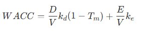
Where D/Vand E/V represent the target market-value weights of debt and equity, respectively; kd is the cost of debt; ke is the cost of equity; and Tm is the company’s marginal tax rate.

Each of WACC’s primary components is directly governed by market-pricing dynamics:

The Cost of Equity (ke) and Systematic Risk: Estimated primarily via the Capital Asset Pricing Model (CAPM), the cost of equity adjusts the expected return of the overall stock market for the risk of the specific company. Because investors can easily eliminate unique, company-specific (idiosyncratic) risks by holding a diversified portfolio of securities, the market does not compensate investors for these risks. WACC is therefore driven strictly by nondiversifiable (systematic) risk, which is measured by a stock’s beta.
The Cost of Debt (kd) as a Promised Yield: For investment-grade firms, the cost of debt is approximated using the yield to maturity (YTM) of its long-term, option-free bonds, representing the current market price of debt. The book warns that coupon rates are historical artifacts set at the time of issuance and are entirely irrelevant for WACC.
Target Market-Value Weights: To weight debt and equity, analysts must use forward-looking target market-value weights rather than book values. Book value is a sunk cost and carries no economic relevance for current investment decisions. Furthermore, current market weights are utilized because today’s capital structure can temporarily swing away from the strategic targets management expects to maintain over the long run.
Operating Liabilities Exclusion: WACC strictly excludes the expected returns of operating liabilities, such as accounts payable. Supplier-provided capital is already compensated through implicit interest embedded in the cost of goods sold, meaning its cost is already deducted before arriving at the free cash flows being discounted.

2. The Interest Tax Shield and Operating Independence

A key strategic choice in corporate finance is separating operating decisions from financing decisions. To allow managers and investors to compare the core profitability of different businesses on an apples-to-apples basis, Free Cash Flow (FCF) is calculated as if the company were financed entirely with equity.

Consequently, the tax savings generated by tax-deductible interest payments—the interest tax shield—are excluded from FCF. Instead, the enterprise DCF model values the interest tax shield by reducing the cost of debt in the WACC formula by the marginal tax rate: kd(1−Tm).

3. Key Structural Assumptions and Limitations of WACC

Within the broader universe of valuation frameworks, WACC-based models are highly intuitive but carry strict structural assumptions:

The Constant Leverage Assumption: Discounting all future cash flows with a constant WACC implicitly assumes that the company actively manages its capital structure to keep its debt-to-value ratio constant over time.
WACC vs. Adjusted Present Value (APV): If a company plans to alter its capital structure significantly (such as paying down a mountain of debt in a leveraged buyout), its debt-to-value ratio will shift annually, violating WACC’s constant leverage assumption. Adjusting WACC year-by-year is mathematically complex and prone to errors. In these dynamic situations, the book recommends using the APV model, which discounts operating cash flows at the unlevered cost of equity and values the tax shields separately.
WACC vs. Cash Flow to Equity (CFE): Unlike enterprise WACC-based models, which value equity indirectly by subtracting debt from enterprise value, CFE models value equity directly by discounting cash flows to equity at a levered cost of equity. The book generally advises against CFE because it is highly sensitive to implicit, unadjusted changes in leverage and distorts the valuation of low-risk nonoperating assets like excess cash by discounting them at a high cost of equity.

Ultimately, while estimating WACC with absolute precision is highly difficult due to unobservable market expectations, the book notes that corporate value is primarily driven by operating strategy. For most companies, the wide variation in Return on Invested Capital (ROIC) across projects has a far greater impact on value creation than minor, hotly debated fluctuations in the WACC.

Enterprise Value to Value per Share

In the larger context of capital and market pricing, the book emphasizes that converting core operating value into value per share is a critical, multi-step process. This process bridges the gap between a company’s internal cash-generating power (the value of operations) and the pricing of claims in the external capital markets.

To align with the principles of market pricing, the book mandates that all weightings, asset values, and claims must be calculated on a current market-value basis rather than using book values, as book values represent sunk costs that do not reflect today’s opportunity cost of capital.

1. From Core Operating Value to Enterprise Value

The buildup process begins with the discounted-cash-flow (DCF) value of core operations. To determine the total Enterprise Value (representing the value of the entire company), you must add the market value of all nonoperating assets:

Excess Cash and Marketable Securities: While some cash is needed to run a business, cash held above this operational requirement is treated as a nonoperating asset. The book suggests a rule of thumb estimating required operating cash at 2 percent of revenues, with any cash above this threshold designated as excess and valued at fair market value.
Investments in Nonconsolidated Companies (Equity Stakes): For minority stakes (typically 20 to 50 percent ownership under the equity method, or below 20 percent under the cost method), the subsidiary’s revenues and costs are not consolidated on the parent’s financial statements. Their value is not captured in free cash flow, so they must be valued separately (using market stock prices for public companies or separate DCF/multiple analyses for private firms) and added.
Tax Loss Carryforwards: These represent future tax savings that should be projected, discounted at the Weighted Average Cost of Capital (WACC), and added as nonoperating assets.

Note on Definition: The book explicitly distinguishes its definition of Enterprise Value (Value of Operations + Nonoperating Assets) from the common investment banking definition (Debt + Equity − Cash). The banking definition is only equivalent if a company has no other nonoperating assets (like joint ventures) or debt equivalents (like pension shortfalls), otherwise it can lead to severe valuation distortions.

2. From Enterprise Value to Equity Value

To isolate the value belonging strictly to common shareholders, the book requires subtracting all nonequity claims from the Enterprise Value. Nonequity claims are financial claims against enterprise value whose expenses are not included in EBITA and are consequently excluded from free cash flow. These claims must be valued at current market rates or market-consistent option-pricing models rather than book values:

Interest-Bearing Debt: Includes short-term and long-term debt, valued at current market prices (via databases like TRACE) or by discounting promised payments at current yields for comparably rated debt.
Debt Equivalents: These include capitalized operating leases, environmental remediation liabilities, and unfunded pension or postretirement obligations. For example, unfunded pension shortfalls should be treated as a debt equivalent and deducted after-tax.
Hybrid Securities: Convertible debt, convertible preferred stock, and employee stock options possess characteristics of both debt and equity. Because their values are highly dependent on the enterprise value, they must be valued using option-pricing models (such as the Black-Scholes model) rather than book values.
Noncontrolling Interests: If a third party holds a minority stake in a consolidated subsidiary, the proportional value owned by outsiders represents a prior claim on cash flow and must be deducted.

The Danger of Double-Counting

The book strongly warns against double-counting nonequity claims. If you deduct a pension shortfall or operating lease liability as a debtlike claim from the enterprise value, you must not also model those pension cash contributions or lease outflows within your free cash flow projections. Doing so would systematically penalize and underestimate the equity value.

3. Deriving Value per Share

The final step is converting the residual equity value into the intrinsic value per share.

The Undiluted Shares Rule: If convertible debt, convertible preferred stock, and outstanding employee stock options have been valued separately and subtracted as nonequity claims, you must divide the equity value by the current number of undiluted shares outstanding. Using diluted shares in this scenario would double-count the dilutive impact of the options and artificially depress the value per share.
The Diluted Shares Exception: If you chose to use the simplified “conversion value” or “exercise value” approaches to handle convertibles and employee options (assuming immediate exchange/exercise and adding option proceeds to equity), then you must divide the equity value by the diluted number of shares.

Ultimately, the book notes that walking through this disciplined, sequential buildup ensures that managers do not make poor strategic decisions—or become vulnerable to hostile takeovers and activist attacks—based on misunderstandings of how market pricing translates enterprise value into value per share.

Multiples Analysis

The book explains that multiples are not a shortcut to valuation, but a relative-valuation check that must be rigorously aligned with the economic principles of cash flow, growth, and cost of capital. When viewed in the larger context of capital and market pricing, a company’s valuation multiple is not arbitrary; it is mathematically derived from the same fundamental value drivers that govern a discounted cash flow (DCF) model—namely, expected Return on Invested Capital (ROIC), revenue growth (), and the Weighted Average Cost of Capital (WACC).

1. Market Pricing of Leverage and Capital Structure (Why to Avoid P/E)

A common mistake made by managers is relying on the Price-to-Earnings (P/E) multiple to compare valuations. The book warns that P/E is heavily distorted by a company’s capital structure because it commingles operating performance with financing risk:

The Cost of Equity Effect: Shifting from equity to debt financing does not create value under the conservation of value principle. Instead, carrying more debt increases financial leverage, which raises the risk borne by shareholders.
Depressed Multiples: To compensate for this heightened risk, the market demands a higher expected return (cost of equity), which drives down the company’s P/E multiple—meaning each dollar of earnings is worth less to an investor. Only for extremely high-growth firms will P/E rise with leverage [794, 856n1].
Enterprise Multiples as the Solution: To compare core operating performance on an apples-to-apples basis, analysts should use Enterprise Value (EV) to EBITA or NOPAT multiples. These multiples are independent of a company’s financing choices and focus solely on the value generated by core operations.

2. Market Pricing of Corporate Taxes (NOPAT vs. EBITA)

Capital markets price the impact of cash taxes, meaning that pre-tax multiples can lead to serious mispricings when comparing companies across different tax environments:

Tax Rate Distortions: Pre-tax multiples like EV/EBITA fail to capture the value-destroying effect of high tax rates. For instance, a company operating in France with a high tax rate cannot be compared cleanly to one in Ireland with a low tax rate using pre-tax EBITA.
Corporate Structure Pricing: The market’s pricing of tax differences was historically demonstrated by U.S. pipeline companies. While pipeline C-corporations (subject to corporate income tax) traded at EBITA multiples of 13 to 14 times, Master Limited Partnerships (MLPs, which pay no corporate taxes) traded at 19 to 25 times. When valued using post-tax NOPAT multiples, both structures traded in a narrow, consistent range of 19 to 25 times.
NOPAT Superiority: Therefore, when peer companies face different tax rates or structures, the book dictates using net enterprise value to NOPAT multiples to maintain consistency with market pricing.

3. Consistency in Market Value Adjustments (Net Enterprise Value)

To reflect the true pricing of core operating assets, the numerator of the multiple must consist strictly of net enterprise value. This requires adjusting the market values of all nonoperating assets and liabilities so they perfectly align with the earnings listed in the denominator:

Subtracting Nonoperating Assets: Assets that do not contribute to EBITA or NOPAT—such as excess cash and nonconsolidated subsidiaries (equity investments)—must be valued at their current market rates and subtracted from the gross enterprise value. For example, failing to subtract Oracle’s $38 billion in cash would systematically distort its operating multiple upward from 11.3 to 13.3 times.
Adding Nonequity Claims: Conversely, claims that are supported by EBITA but not held by common shareholders—such as noncontrolling interests—must be valued and added to the enterprise value calculation to avoid biasing the multiple downward.

4. Market Pricing of Industry Peers (Peer Group Selection)

A fundamental tenet of market pricing is that similar assets with similar risk and return profiles must sell for similar prices. However, the book notes that broad industry averages are too noisy for relative valuation. A proper peer group must consist of close competitors that share identical performance expectations:

ROIC and Growth Alignment: Since multiples are mathematically derived from ROIC and growth, peer groups must be segmented by these key value drivers. Comparing a low-ROIC, low-growth company against a high-ROIC, high-growth industry leader will suggest an artificial “undervaluation” or a “conglomerate discount” when, in reality, it is simply a performance discount.
Deficiencies of the PEG Ratio: While the Price-to-Earnings-to-Growth (PEG) ratio attempts to control for growth, it is seriously deficient because it ignores ROIC. A high-ROIC firm will naturally trade at a higher PEG than a low-ROIC firm with identical growth, meaning a simple PEG comparison will mistakenly flag the superior value creator as “overvalued”.

Valuation by Parts

In the book, valuing a multibusiness company as a single, consolidated enterprise is described as a practice that frequently leads to inaccurate valuations and poor strategic decisions. Because different business segments compete in distinct markets with vastly different growth prospects, risk profiles, and tax environments, the book establishes Valuation by Parts (Sum-of-the-Parts) as a core technique to isolate and properly value these unique economic units.

When viewed in the larger context of capital and market pricing, Valuation by Parts represents the operational mechanism that ensures every business segment is priced under the exact same risk-return parameters it would face as an independent, stand-alone player in the capital markets.

1. Pricing the Cost of Capital at the Segment Level

A fundamental error in valuing diversified companies is applying a single corporate-wide cost of capital to all business segments. Within the capital pricing framework, the book dictates that each business segment must be valued at its own segment-specific Weighted Average Cost of Capital (WACC):

Unique Risk Profiles: Different segments carry distinct levels of systematic risk (beta) and maintain different capacities to support debt, meaning their WACC must reflect segment-specific capital structures.
Estimating Segment Betas: To price a unit’s equity risk, analysts must identify a peer group of publicly traded pure-play competitors, calculate their levered betas, unlever those betas to isolate pure operating risk, and then relever the median peer beta using the business unit’s target capital structure.
The Irrelevance of Corporate Beta: The book highlights that when a company is valued by summing its parts, there is no need to estimate a corporate-wide cost of capital or reconcile segment betas with the corporate beta. A consolidated corporate beta is highly susceptible to estimation errors and changes dynamically over time as the relative valuation weights of the underlying segments shift. Individual segment WACCs are far more stable and economically meaningful.

2. Pricing and Isolating Financial Subsidiaries

Many large corporations operate customer-finance units that resemble banks rather than standard industrial operations. Because banking economics are highly leveraged and distinct, the book warns that commingling these units with core operations severely distorts corporate ROIC and capital turnover.

To price these units correctly, analysts must value them separately using a Cash-Flow-to-Equity (CFE) model discounted at a bank-specific cost of equity.
When performing the final equity buildup, the book requires extra caution to avoid double-counting the debt of the financial subsidiary. The equity value of the finance unit is already net of its specific funding debt; therefore, when subtracting debt from the total enterprise value to isolate parent equity, only the debt associated with core operating units must be deducted.

3. Market Pricing: Multiples and the “Conglomerate Discount” Illusion

In public equity markets, diversified companies are frequently said to trade at a “conglomerate discount,” prompting activists to demand breakups. However, the book utilizes SOTP and market multiples to prove that the conglomerate discount is almost always a performance discount, not a diversification penalty:

Peer Group Alignment: Traditional sum-of-the-parts calculations conducted by Wall Street often apply broad industry average multiples or multiples of “top-performing” peers to value individual business segments. If a segment underperforms its industry, this top-peer baseline overstates its value, creating a fake valuation gap (or “conglomerate discount”).
Close-Peer Multiples: When segment valuations are instead tested against close-peer multiples (peers possessing similar ROIC and growth profiles), the conglomerate discount completely disappears. If a diversified company trades at a discount to pure-plays, it is because its underlying business units are performing poorly, not because of its corporate structure.
Tax Jurisdiction Distortions: When comparing segments globally or across different tax structures, the book strongly recommends using NOPAT-based multiples instead of EBITA multiples. EBITA-based multiples fail to capture the real market-pricing impacts of varying corporate tax rates across different segments and geographic jurisdictions.

4. SOTP as a Capital Allocation Tool

Ultimately, Valuation by Parts changes how the corporate center interacts with the financial markets. Rather than distributing capital budgets evenly based on historical segment revenues, SOTP equips corporate parents to act like private-equity firms.

By tracking economic profit and value added per dollar of invested capital at the segment level, corporate managers can identify high-return segments where growth will create immense value, versus low-return segments where scaling actually destroys value.
The book notes that companies that actively use these SOTP insights to reallocate capital dynamically away from slow-growth, low-ROIC divisions toward high-value-creating units generate 30 percent higher total shareholder returns (TSR) on average.

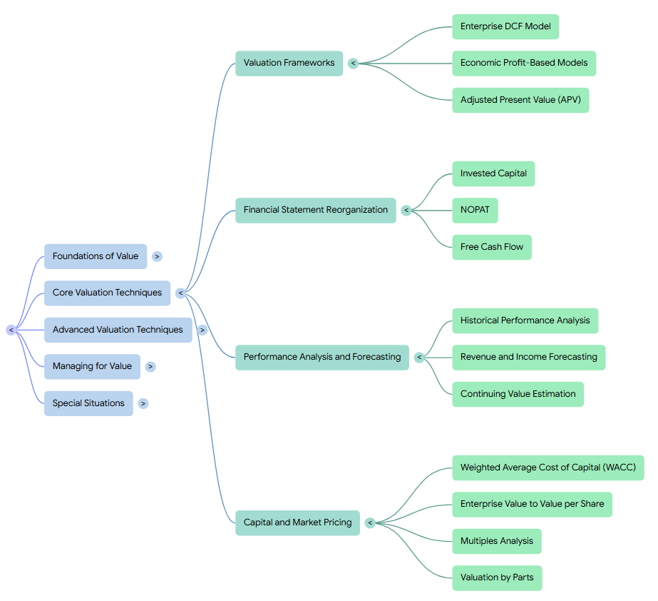
— Linden Lake

This series:
→　Book Review (1 of 5): Valuation – Foundations of Value
→　Book Review (2 of 5): Valuation – Core valuation Techniques
→　Book Review (3 of 5): Valuation – Advanced Valuation Techniques
→　Book Review (4 of 5): Valuation – Managing for Value
→　Book Review (5 of 5): Valuation – Special Situations