Book Review (4 of 5): Financial Statement Analysis – Analysis Tools

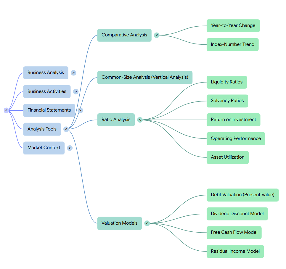
In the book, financial statement analysis is defined as the application of analytical tools and techniques to general-purpose financial statements to derive estimates and inferences useful in business analysis. These tools are designed to reduce reliance on intuition, decrease uncertainty, and provide a systematic basis for evaluating a company’s economic prospects and risks. The book identifies five primary sets of tools for financial analysis: comparative analysis, common-size analysis, ratio analysis, cash flow analysis, and valuation.

Comparative Financial Statement Analysis (Horizontal Analysis)

Comparative analysis involves reviewing consecutive balance sheets, income statements, or statements of cash flows from period to period to identify trends. The book details two primary techniques:

• Year-to-Year Change Analysis: This involves analyzing changes in individual account balances in both absolute dollar amounts and percentages. Using both is necessary to maintain proper perspective on the relative importance of a change.
• Index-Number Trend Analysis: This tool is used for long-term comparisons. An analyst chooses a base period with a preselected index of 100, and all subsequent periods are expressed relative to that base to reveal the direction and speed of a trend.

Common-Size Financial Statement Analysis (Vertical Analysis)

Common-size analysis expresses each financial statement account as a percentage of a significant total, such as total assets for the balance sheet or net sales for the income statement. This is termed “vertical analysis” because it evaluates the internal makeup of a single statement. The book emphasizes its usefulness for:

• Understanding internal structure: Assessing the distribution of financing sources or the composition of assets.
• Intercompany comparisons: Recasting statements of different companies into a common format to highlight differences in account makeup and distribution, regardless of the relative sizes of the firms.

Ratio Analysis

Ratio analysis expresses a mathematical relation between two quantities to gain insights into underlying conditions. The book cautions that ratios are starting points for investigation, not end points, and must refer to economically important relations to be meaningful. Ratios are categorized into three areas:

• Credit (Risk) Analysis: Includes liquidity ratios to evaluate a company’s ability to meet short-term obligations and solvency ratios to assess long-term obligations.
• Profitability Analysis: Focuses on return on investment (ROI), operating performance (profit margins), and asset utilization (turnover).
• Valuation: Used to estimate the intrinsic value of a company or its stock.

Cash Flow Analysis

Cash flow analysis is primarily used as a tool to evaluate the sources and uses of funds. It provides insights into how a company is obtaining its financing and deploying its resources. According to the book, this tool is vital for forecasting cash flows and as a component of liquidity analysis. It also serves as a validator of the quality of accrual-based earnings.

Valuation Models

Valuation is considered a main objective of many types of business analysis. The book states that the theoretical basis for these models is present value theory, which posits that the value of an asset is the sum of all expected future payoffs discounted to the present. Analysts use models such as the dividend discount model, the free cash flow to equity model, or the residual income model to convert forecasted payoffs into an estimate of intrinsic value.

Integration and Context

The book stresses that these tools do not function in isolation; they are part of a larger framework of component processes. Effective use of these tools requires accounting analysis—adjusting reported numbers to better reflect economic reality—before computing ratios or performing valuations. Ultimately, these tools enable an analyst to reconstruct the economic reality embedded in financial statements and make more informed decisions regarding equity, credit, and management.

Comparative Analysis

In the book, comparative financial statement analysis (also known as horizontal analysis) is identified as one of five primary sets of tools for financial analysis, alongside common-size analysis, ratio analysis, cash flow analysis, and valuation. It involves reviewing consecutive financial statements from period to period to identify trends, including their direction, speed, and extent.

Primary Techniques of Comparative Analysis

The book details two especially popular techniques used to perform this analysis:

• Year-to-Year Change Analysis: This is typically used for short-term comparisons of two to three years. It has the advantage of presenting changes in both absolute dollar amounts and percentages. The book emphasizes that viewing both is necessary to maintain a proper perspective on the relative importance of a change; for example, a 50% change from a $1,000 base is far less significant than the same percentage change from a $100,000 base.
• Index-Number Trend Analysis: This tool is used for long-term comparisons. An analyst selects a “normal” base period with a preselected index number of 100, and all subsequent periods for significant items are expressed relative to that base. This technique helps convey insights into managers’ philosophies and how they handle different economic environments.

Analytical Cautions and Rules

The book provides specific guidelines and warnings for conducting effective comparative analysis:

• Computation Constraints: Meaningful percentage changes cannot be computed when a base period has a negative amount and the next is positive (or vice versa), or when there is no amount for the base period.
• Small Base Amounts: Percentages must be interpreted with caution if the base period amount is small, as it can signal a large change that is inconsistent with its actual importance.
• External Factors: Analysts must exercise care when changes might be due to industry or economic factors, price-level changes, or inconsistent applications of accounting principles over time.

Integration with Other Analysis Tools

Comparative analysis is positioned as a foundational process within the larger discipline of financial statement analysis. While it identifies trends in absolute numbers, it is often used in conjunction with common-size (vertical) analysis, which evaluates the internal makeup of a single statement by expressing accounts as a percentage of a significant total. Furthermore, the book stresses that accounting analysis—adjusting reported numbers for better comparability—is an essential prerequisite to performing meaningful comparative analysis. Ultimately, these tools work together to reduce reliance on hunches and decrease the uncertainty of business decisions.

Year-to-Year Change

In the book, year-to-year change analysis is identified as one of the two most popular techniques for performing comparative financial statement analysis (also known as horizontal analysis). This method involves comparing financial statements over relatively short time periods—typically two to three years—by reviewing changes in individual account balances.

The Importance of Duality: Absolute vs. Percentage Changes

A key principle of year-to-year change analysis highlighted in the book is the necessity of presenting changes in both absolute dollar amounts and percentages. The book argues that viewing both is critical for maintaining proper perspective and making valid inferences:

• Contextual Importance: A 50% change from a base of $1,000 is usually far less significant than the same percentage change from a base of $100,000.
• Relative Significance: Reference to the actual dollar amounts ensures the analyst can determine the relative importance of a specific change within the company’s broader financial structure.

Computational Rules and Constraints

The book details specific rules that govern the computation of these changes to ensure they remain meaningful:

• Negative to Positive Shifts: If a base period has a negative amount and the next period is positive (or vice versa), a meaningful percentage change cannot be computed.
• Zero Base Amounts: No percentage change can be calculated if there is no amount for the base period.
• Small Base Amounts: Percentages derived from very small base amounts must be interpreted with extreme caution, as they can signal a massive change that is inconsistent with its actual economic importance.
• Full Decreases: When an account has a value in the base period but none in the following period, the decrease is recorded as 100%.

Analytical Applications and Inferences

Beyond individual line items, the book explains that comparative analysis is used to evaluate trends in interrelated items. For instance:

• Sales vs. Costs: If a 10% increase in sales is accompanied by a 20% increase in freight-out costs, it requires further investigation to understand the discrepancy.
• Sales vs. Receivables: Similarly, a 15% increase in accounts receivable alongside a mere 5% increase in sales suggests potential issues with collection or credit policy.

Example: Colgate’s Comparative Results

The book illustrates these concepts using Colgate’s income statements for 2010 and 2011. The year-to-year analysis revealed that while net sales increased by 7.5%, the cost of sales surged by 12.3%. Because the cost increase outpaced revenue growth, the resulting increase in gross profit was only 4.2%. This specific comparison allowed analysts to infer that Colgate was operating with increasing production costs that were compressing its margins despite higher sales volume.

Ultimately, this technique serves as a foundational tool within the larger framework of financial analysis to identify the direction, speed, and extent of trends, thereby reducing reliance on intuition and guesswork.

Index-Number Trend

In the book, index-number trend analysis is identified as one of the two most popular techniques for conducting comparative financial statement analysis, specifically designed for long-term comparisons. While year-to-year change analysis is effective for short periods of two to three years, the book notes that it becomes cumbersome for longer durations, making index-number trends a more useful tool for identifying the direction, speed, and extent of trends over many periods.

Methodology and Computation

The process of index-number trend analysis involves several specific steps and rules:

• Base Period Selection: An analyst must first choose a “normal” base period for all items, which is assigned a preselected index number typically set to 100.
• Relative Expression: All subsequent periods for significant financial statement items are then expressed as a percentage relative to that base period.
• Formula: The index for a current year is computed by dividing the current year balance by the base year balance and multiplying by 100.
• Percentage Changes: The book cautions that while changes relative to the base year are easily inferred, percentage changes between subsequent non-base years must be computed by referencing the previous year’s balance or through a ratio of their index numbers.
• Constraints: Similar to other comparative methods, meaningful index numbers cannot be expressed when an item shifts from a negative to a positive amount (or vice versa).

Analytical Cautions

The book emphasizes that index-number trend analysis requires careful interpretation and should not be applied blindly to every line item. Analysts should focus on significant items and exercise care if changes are primarily driven by broader economy or industry factors rather than company-specific performance. Furthermore, the book stresses that an analyst must be aware of potentially inconsistent applications of accounting principles over time and the distortive effects of price-level changes (inflation) when comparing data over very long periods.

Strategic Insights

Beyond simple numerical comparisons, the book highlights that the primary power of trend analysis is its ability to convey insights into managers’ philosophies, policies, and motivations. By examining how a company handles diverse economic environments over time—such as periods of adversity or opportunity—the analyst can form a better picture of management’s effectiveness.

For example, the book illustrates this using Colgate’s results from 2006 to 2011, where an index-number trend analysis revealed that while sales growth slowed between 2008 and 2010, the company successfully slowed the increase in operating expenses to maintain a growth trend in net income. Ultimately, this tool helps reduce reliance on intuition and guesswork by providing a systematic basis for evaluating long-term prospects.

Common-Size Analysis (Vertical Analysis)

In the book, common-size financial statement analysis (also referred to as vertical analysis) is identified as one of the five primary sets of tools used in financial analysis. It is characterized by expressing each individual financial statement account as a percentage of a significant total—total assets for the balance sheet and net sales for the income statement. This technique is termed “vertical” because it evaluates the internal makeup and distribution of accounts within a single statement.

Strategic Use of Common-Size Analysis

The book emphasizes that common-size analysis is vital for understanding the internal structure of an enterprise through two primary lenses:

• Sources of Financing: On the balance sheet, it reveals the distribution of a company’s financing across current liabilities, noncurrent liabilities, and equity. For example, the analysis of Colgate reveals that a “lion’s share” of its financing is debt, with total liabilities reaching 80% of assets.
• Composition of Assets: It allows analysts to evaluate the mix of a company’s resources, such as the proportion of current versus noncurrent assets. In the case of manufacturing companies like Colgate, common-size analysis shows that property, plant, and equipment (PP&E) typically constitute a significant portion (roughly 30%) of total assets.

Analytical Applications and Inferences

Within the income statement, each expense item is related to sales to determine what percentage of every dollar earned is consumed by specific costs. The book notes that while sales impact nearly all expenses, an exception is income taxes, which should be related to pre-tax income for a more meaningful analysis.

Furthermore, the book highlights two specific types of comparisons enabled by this tool:

• Intertemporal Comparisons: Comparing a single company’s common-size statements over several years reveals proportionate changes in account makeup across time.
• Intercompany Comparisons: The book stresses that common-size statements are “especially useful” for comparing companies of different sizes. By recasting financial data into a common percentage format, analysts can highlight differences in account distribution and competitive strategy regardless of the relative size of the firms.

Analytical Cautions and Limitations

The book provides a critical warning for those using vertical analysis: percentages must be interpreted with an examination of the absolute dollar amounts. A percentage might decline not because the account balance itself decreased, but because the total category (the base) increased at a faster rate. Additionally, while excellent for comparing the mix of assets or expenses, common-size statements fail to reflect the relative scale of the companies under analysis.

Integration with Other Analysis Tools

In the larger framework of business analysis, common-size analysis is often used in tandem with comparative (horizontal) analysis to provide a complete picture of both absolute trends and relative structural changes. It serves as a foundational component in several “building blocks” of analysis, such as evaluating capital structure and solvency and assessing operating performance. Consistent with this, the book applies common-size analysis to both Colgate and Campbell Soup to provide a detailed evaluation of their long-term financial health and profitability.

Ratio Analysis

In the book, ratio analysis is identified as one of the five primary sets of tools for financial analysis, alongside comparative analysis, common-size analysis, cash flow analysis, and valuation. It is defined as a method of expressing a mathematical relation between two quantities to gain insights into a company’s underlying conditions.

The Nature and Logic of Ratios

The book emphasizes that while the arithmetic of a ratio is simple, its interpretation is complex. For a ratio to be meaningful, it must refer to an economically important relation, such as the direct link between a product’s sales price and its cost. The book cautions that ratios are merely tools to provide insights and should be viewed as starting points for investigation rather than end points. To be most effective, ratios should be future-oriented, meaning analysts often adjust the factors affecting them for their probable future trends and magnitudes.

Primary Areas of Ratio Analysis

The book categorizes ratios into three fundamental areas of financial statement analysis:

• Credit (Risk) Analysis: This includes liquidity ratios to evaluate a company’s ability to meet short-term obligations and capital structure and solvency ratios to assess long-term debt-paying ability.
• Profitability Analysis: This focuses on return on investment (ROI) to assess financial rewards to providers of capital, operating performance to evaluate profit margins, and asset utilization (turnover) to assess the effectiveness of assets in generating sales.
• Valuation: These ratios are used to estimate the intrinsic value of a company or its stock.

Factors Affecting Interpretation

The book highlights several critical factors that analysts must consider to use ratios effectively:

• Prerequisite Accounting Analysis: Before computing ratios, it is essential to perform accounting analysis to ensure the underlying numbers are reliable and appropriate. For instance, the use of LIFO inventory valuation during periods of rising prices can understate the current ratio.
• Comparative Context: Ratios are rarely relevant in isolation; they must be interpreted in comparison with a company’s own prior ratios, predetermined standards, or the ratios of competitors.
• Correlated Variables: Analysts must be careful because factors affecting the numerator can correlate with those in the denominator. For example, a company might improve its ratio of operating expenses to sales by cutting advertising costs, but this action could lead to long-term declines in sales and market share.
• Variability and Trend: The book notes that the variability of a ratio over time is often just as important as its general trend.

Ultimately, the book argues that the usefulness of ratio analysis depends on the skill of the analyst in applying and interpreting these measures within the broader context of economic events, industry factors, and management policies.

Liquidity Ratios

In the book, liquidity ratios are identified as a fundamental component of ratio analysis, specifically categorized under credit (risk) analysis. While ratio analysis is one of the five primary sets of tools for financial statement analysis, liquidity ratios focus specifically on evaluating a company’s ability to meet its short-term financial obligations and react to unexpected interruptions in the flow of funds.

The Role of Liquidity Ratios in Analysis

The book emphasizes that liquidity ratios should be viewed as a “starting point” for investigation rather than an end point. Within the larger context of business activities, these ratios help analysts determine the “nearness to cash” of a company’s assets and liabilities. A lack of liquidity can be a precursor to more severe financial distress, potentially leading to the forced sale of assets or, in extreme cases, insolvency and bankruptcy.

Primary Liquidity Ratios

The book details several key mathematical relations used to gain insights into short-term solvency:

• Current Ratio: Calculated as current assets divided by current liabilities, this is the most common measure of current liability coverage.
• Acid-Test (Quick) Ratio: A more stringent test that includes only the most liquid assets (cash, cash equivalents, marketable securities, and receivables) in the numerator.
• Asset Utilization Measures: These determine the speed at which non-cash assets are converted into cash. Key ratios include accounts receivable turnover and inventory turnover, as well as their counterparts in days (the collection period and days to sell inventory).
• Cash-Based Ratios: These measures, such as the cash ratio to current assets or the cash flow to current liabilities ratio, provide a dynamic view of liquidity by relating cash flows directly to short-term obligations.

Factors Affecting Interpretation

The book highlights that the arithmetic of a liquidity ratio is simple, but its interpretation within the context of ratio analysis is complex:

• Prerequisite Accounting Analysis: Before computing these ratios, an analyst must perform accounting analysis to ensure the underlying numbers are appropriate. For example, the use of LIFO inventory valuation can significantly understate a company’s current ratio during periods of rising prices.
• The Operating Cycle: Liquidity ratios must be interpreted in light of a company’s net trade cycle and industry norms. What is considered a healthy ratio in one industry may signal inefficiency or distress in another.
• Comparative Context: Ratios are rarely meaningful in isolation and should be compared against the company’s own historical trends, predetermined standards, or the ratios of competitors.
• Static vs. Dynamic Measures: The book cautions that many liquidity ratios (like the current ratio) are static snapshots at a point in time. To get a complete picture, they must be supplemented with dynamic measures like cash flow analysis.

Ultimately, the book positions liquidity ratios as essential screening devices that direct an analyst to areas of greatest change or unexplained performance, helping to reduce reliance on hunches and intuition in credit decisions.

Solvency Ratios

In the book, solvency ratios are identified as a vital component of credit (risk) analysis, which is one of the primary areas of ratio analysis. While liquidity ratios focus on short-term obligations, solvency ratios evaluate a company’s long-run financial viability and its ability to meet long-term commitments.

The Role of Solvency Ratios in Analysis

The book emphasizes that solvency depends on both a company’s capital structure and its long-term profitability. Within the broader framework of ratio analysis, solvency measures serve as “screening devices” that help analysts decide if the risk inherent in a company’s financing requires deeper investigation. These ratios are generally divided into two categories: capital structure measures and earnings coverage measures.

Primary Capital Structure Ratios

These ratios relate different components of a company’s financing sources to one another to measure financial risk and leverage:

• Total Debt to Total Capital (Total Debt Ratio): Measures the proportion of total assets financed by all forms of debt.
• Total Debt to Equity Capital: Compares the total credit financing to the total equity financing provided by owners.
• Long-Term Debt to Equity Ratio (Debt to Equity Ratio): Measures the relationship between noncurrent liabilities and equity capital; a ratio exceeding 1:1 indicates that long-term debt financing outweighs owner financing.

Earnings Coverage Ratios

Because capital structure ratios do not account for the availability of cash flows to service debt, the book highlights earnings coverage ratios as a crucial secondary measure of solvency:

• Times Interest Earned: A simplified measure that considers interest as the only fixed charge needing coverage by earnings.
• Earnings to Fixed Charges: A more comprehensive formula that includes interest, lease rentals, and other fixed commitments in the denominator.
• Cash Flow to Fixed Charges: A dynamic measure that relates pretax operating cash flow to fixed charges, recognizing that obligations are paid with cash rather than accrual earnings.

Factors Affecting Interpretation

Like all tools in ratio analysis, the book cautions that solvency ratios should not be viewed in isolation:

• Earnings Variability: Companies in stable industries (like utilities) can safely maintain lower coverage ratios than cyclical companies (like machinery manufacturers).
• Accounting Adjustments: Analysts must often adjust book values for items like operating leases, off-balance-sheet financing, and deferred taxes to arrive at a “true” measure of debt and equity.
• Industry Benchmarks: Acceptable levels for these ratios vary significantly across industries, and a company should be benchmarked against its competitors to assess its relative risk.
• The Double-Edged Sword of Leverage: While debt can increase returns to shareholders through financial leverage, excessive debt limits management’s flexibility and increases the risk of default during economic downturns.

Return on Investment

In the book, Return on Investment (ROI)—also referred to as Return on Invested Capital (ROIC)—is identified as one of the three fundamental areas of ratio analysis, alongside credit risk analysis and valuation. It is described as probably the most widely recognized measure of company performance, providing a comprehensive basis for comparing companies’ success in using their level and source of financing to generate profits.

The Role of ROI in Ratio Analysis

While the arithmetic of an ROI ratio is simple, the book emphasizes that its interpretation is complex because it must refer to economically important relations to be meaningful. ROI ratios serve three critical purposes in business analysis:

• Measuring Managerial Effectiveness: It reflects the skill and resourcefulness of management in making financing, investing, and operating decisions.
• Assessing Profitability: It acts as a vital indicator of long-term financial strength, relating summary measures from both the income statement and balance sheet.
• Planning and Control: ROI helps management exercise control over individual profit centers and evaluate the returns achieved by specific projects or divisions.

Primary ROI Measures

The book distinguishes between two main measures of ROI based on different definitions of invested capital:

1. Return on Net Operating Assets (RNOA)

RNOA measures the after-tax profit earned specifically from a company’s core operating activities. It is computed as Net Operating Profit After Tax (NOPAT) divided by average Net Operating Assets (NOA). The book explains that RNOA can be disaggregated into two key drivers:

• Net Operating Profit Margin: Measuring profitability relative to sales.
• Net Operating Asset Turnover: Measuring the effectiveness in generating sales from assets. This decomposition allows analysts to see if a company achieves its return through high margins, high volume, or a mix of both.

2. Return on Common Equity (ROCE)

ROCE is of primary interest to shareholders as it measures the residual earnings available to them after all other financing sources are paid. It is computed as (Net Income – Preferred Dividends) divided by average Common Shareholders’ Equity. The book disaggregates ROCE to show it is a function of both operating performance and financial strategy:

• ROCE=RNOA+(Financial Leverage × Spread). This formula reveals how much of the return is derived from core operations versus how much is boosted (or reduced) by the company’s use of debt.

Analytical Considerations

The book stresses that before computing ROI ratios, an analyst must perform accounting analysis to ensure the underlying numbers accurately reflect economic reality. For example, the use of LIFO inventory valuation can understate the asset base, while unrecorded liabilities like operating leases can distort both the numerator and denominator of ROI measures. Additionally, the book notes that because ROI ratios tend to revert to long-run averages over time due to competition, analysts should assess them over a full business cycle rather than relying on a single year’s results.

Operating Performance

In the book, operating performance analysis is identified as one of the three fundamental areas of ratio analysis, specifically categorized under the broader umbrella of profitability analysis. While ratio analysis as a whole expresses mathematical relations to gain insights into a company’s underlying conditions, operating performance ratios focus specifically on evaluating profit margins derived from a company’s earning-related activities.

Key Ratios for Operating Performance

Operating performance is primarily assessed through ratios that link income statement line items to net sales, often referred to collectively as profit margins. The book identifies several critical measures:

• Gross Profit Margin: Calculated as (Sales – Cost of Sales) / Sales, this ratio measures a company’s inherent ability to sell its products or services well above the cost of production.
• Operating Profit Margin (Pretax): Computed as Operating Income / Sales, this reflects the profitability of normal business operations before considering financing costs and taxes.
• Net Profit Margin: Calculated as Net Income / Sales, this represents the “bottom line” profitability for every dollar of revenue earned.

Analytical Purpose and Interpretation

The book emphasizes that these ratios are comparable to the results of common-size income statement analysis, as both evaluate the internal makeup of the income statement relative to sales. From an analytical perspective, these measures reflect the skill and resourcefulness of management in making operating decisions. For example, a high gross profit margin provides the necessary “cushion” to finance essential future-directed discretionary expenditures such as research and development or advertising. Conversely, a declining margin may signal that a company is operating in an intensely competitive environment or facing surging production costs that it cannot pass on to consumers.

Integration and Disaggregation

Within the larger context of ratio analysis, operating performance is closely linked with asset utilization (turnover), as both are key drivers of a company’s total return on investment. To gain deeper insights, the book suggests disaggregating the pretax profit margin into its various components—such as selling, administrative, and research expenses relative to sales—to identify the specific factors driving changes in profitability. Ultimately, these ratios serve as “starting points” for investigation, directing analysts to areas of unexplained performance or significant changes in a company’s competitive position.

Asset Utilization

In the book, asset utilization analysis (also referred to as turnover analysis) is identified as one of the three fundamental pillars of ratio analysis under the broader category of profitability analysis. While ratio analysis expresses mathematical relations to gain insights into a company’s conditions, asset utilization specifically measures the “intensity” and “effectiveness” with which a company uses its assets to generate sales.

The Role of Asset Utilization in Profitability

The book emphasizes that asset utilization is a primary determinant of a company’s Return on Invested Capital (ROIC). Specifically, the Return on Net Operating Assets (RNOA) is disaggregated into two components:

1. Net Operating Profit Margin: Profitability relative to sales.
2. Net Operating Asset Turnover: The effectiveness of generating sales from those assets.

This relation is central to a company’s strategy; for example, a supermarket may have a low profit margin but achieve a high RNOA through very high asset turnover.

Primary Asset Utilization Ratios

The book details several specific ratios used to evaluate the productivity of different asset categories:

• Accounts Receivable Turnover: Calculated as NetSales/AverageAccountsReceivable. It measures the speed of collections. A low turnover (or a long average collection period) can signal poor collection efforts or customers in financial distress.
• Inventory Turnover: Calculated as Calculated as Cost of Goods Sold/Average Inventory. This ratio uses cost of goods sold rather than sales because inventory is reported at cost. A decline often suggests uncompetitive products or obsolescence.
• Long-Term Operating Asset Turnover: Sales/Average Long−Term Operating Assets. This is particularly relevant for capital-intensive manufacturing companies.
• Net Operating Working Capital Turnover: Net Sales/Average Net Operating Working Capital. This reflects how much investment in working capital is required for each dollar of sales.

Analytical Interpretation and Limitations

The book provides several cautions for interpreting these ratios within the context of financial statement analysis:

• Optimization vs. Minimization: While higher turnover is generally better, the book warns against “minimizing” assets to the point of hurting the business. For example, a restrictive credit policy might increase receivables turnover but lead to lost sales.
• Operating Cycle (Conversion Period): Analysts often combine receivables and inventory turnover to determine the total time required to convert non-cash assets into cash.
• Impact of Accounting Methods: The book stresses that accounting analysis must precede ratio computation. For instance, using LIFO inventory valuation during inflationary periods can result in artificially high inventory turnover ratios because the inventory base (the denominator) is reported at outdated, lower costs.
• Industry Comparisons: Asset utilization varies significantly by industry. For example, the book notes that Campbell Soup’s inventory turnover (8.8) is much higher than the industry composite (3.6), reflecting more efficient management of raw materials and finished goods.

Valuation Models

In the book, valuation is identified as one of the five primary sets of tools for financial statement analysis, alongside comparative, common-size, ratio, and cash flow analysis. It is considered a main objective of many types of business analysis, serving as the process of converting forecasts of future payoffs into an estimate of a company’s intrinsic value.

Theoretical Foundation: Present Value Theory

The book states that the theoretical basis for valuation is present value theory, which posits that the value of an asset is equal to the sum of all its expected future payoffs, discounted to the present at an appropriate discount rate. To implement this, an investor requires two pieces of information:

• Expected Future Payoffs: For bonds, these are interest and principal; for stocks, these are dividends and capital appreciation.
• Discount Rate: For bonds, this is the yield to maturity; for stocks, it is the risk-adjusted cost of capital.

Primary Valuation Models

While several models exist, the book highlights three specific approaches for valuing equity:

• Dividend Discount Model (DDM): This model defines the value of an equity security as the sum of the present values of all future expected dividends. However, it faces practical obstacles because dividends are discretionary and forecasting them over an infinite horizon is difficult.
• Free Cash Flow to Equity (FCFE) Model: This model replaces expected dividends with expected free cash flows to equity. Free cash flows to equity are defined as cash flows from operations minus capital expenditures, plus or minus changes in debt.
• Residual Income Model: This model computes value using accounting variables, defining equity value as the sum of current book value and the present value of all future expected residual income. Residual income is defined as comprehensive net income minus a charge on the beginning book value (reflecting the cost of capital).

Practical Application and “Value Drivers”

The book emphasizes that while all three models—DDM, FCFE, and RI—are mathematically identical and exact over an infinite horizon, they differ in a finite horizon setting. In practice, analysts typically use a finite forecast horizon (e.g., five to ten years) and must then estimate a continuing value (or terminal value) to account for payoffs beyond that period.

The residual income model is often preferred because it is least dependent on the continuing value estimate and focuses on “value drivers” such as Return on Equity (ROE). In equilibrium, competitive forces tend to drive ROE toward the cost of capital; valuation, therefore, involves projecting the rate at which a company’s ROE reverts to this long-run equilibrium.

Integration with Other Analysis Tools

In the larger context of financial statement analysis, valuation is the culmination of prospective analysis, which involves forecasting future payoffs. Before performing a valuation, the book stresses that an analyst must first conduct accounting analysis (to ensure the reliability of the reported numbers) and financial analysis (to assess the company’s track record and profitability drivers). These combined tools enable the analyst to “reconstruct the economic reality” embedded in the financial statements to reach a defensible estimate of company value.

Debt Valuation (Present Value)

In the book, debt valuation is presented as an application of present value theory and serves as a foundational concept for understanding more complex valuation models,. Because a bond contract precisely specifies future payoffs and the investment horizon, debt valuation provides a straightforward setting for grasping the mechanics of intrinsic value estimation,.

Theoretical Foundation: Present Value Theory

The book states that the theoretical basis for all valuation is present value theory, which posits that the value of any security is equal to the sum of all its expected future payoffs, discounted to the present at an appropriate rate,. This theory is rooted in the concept of the time value of money—the idea that an entity prefers consumption in the present over consumption in the future.

Essential Information for Debt Valuation

To value a debt security, the book specifies that an investor requires two primary pieces of information:

• Expected Future Payoffs: For bonds, these consist of periodic interest (coupon) payments and the eventual repayment of the principal (face value) at maturity,.
• Discount Rate: In the case of debt, the discount rate is the prevailing interest rate, specifically referred to as the yield to maturity,. This rate is determined by factors such as current market interest rates, expected inflation, and the specific risk of default associated with the borrower.

The Bond Valuation Formula

The book provides a formal mathematical formula to calculate the value of a bond at a specific time (B_t). The value is determined by discounting each individual interest payment (I) and the final principal payment (F) by the required interest rate (r) over the number of periods (n) until they are received:

Context within Valuation Models

Within the larger context of valuation, the book distinguishes debt valuation from equity valuation based on the certainty of these variables. While the basis for both is the present value of future payoffs, equity valuation is significantly more complex because investors have no claim on predetermined payoffs; instead, they must forecast uncertain future dividends and capital appreciation,. Consequently, while a bond’s value can be computed with relative precision based on its contract, the valuation of equity depends on the analyst’s ability to forecast future performance and determine a risk-adjusted cost of capital,.

Dividend Discount Model

In the book, the dividend discount model (DDM) is presented as a fundamental approach for estimating the intrinsic value of a company’s equity. It is rooted in present value theory, which posits that the value of any security—debt or equity—is equal to the sum of all its expected future payoffs, discounted to the present at an appropriate rate.

Definition and Theoretical Basis

The book defines the value of an equity security at a specific time (V_t​) as the sum of the present values of all future expected dividends. While equity investors also look for capital appreciation, the book explains that capital appreciation is itself determined by future dividends, allowing the valuation task to be simplified into this single formula:

In this model, E(D_t+n​)represents the expected dividend in period , and represents the cost of equity capital. The book emphasizes that this formula uses forecasts of future dividends because, unlike the interest payments on a bond, dividends are not specified by contract and cannot be determined with certainty.

Context within Valuation Models

The DDM is one of three primary models discussed in the book for valuing equity, alongside the free cash flow to equity (FCFE) model and the residual income model. While the book notes that these three models are mathematically identical and exact over an infinite horizon, they often yield different results when applied in practice over a finite period. In a comparative illustration, the book demonstrates that if terminal values are set (such as in an acquisition scenario), all three models will yield the same intrinsic value.

Practical Obstacles and Limitations

Despite its theoretical soundness, the book identifies several significant practical obstacles to using the DDM:

• Infinite Horizon: Practically, analysts must compute value using a finite forecast horizon, and forecasting dividends indefinitely is difficult.
• Management Discretion: Dividends are discretionary. The book points out that different companies adopt different payout policies; some may reinvest most earnings for growth while others pay them out, meaning actual dividend payouts are not always indicative of a company’s total value in the short to medium term.
• Comparison to Other Models: Because of these difficulties, the book states that analysts often replace dividends with earnings or cash flows in their models. Specifically, the book suggests that the residual income model often outperforms the DDM in finite horizon settings because it is less dependent on the estimation of “continuing value” (terminal value).

Analytical Role

In the larger framework of business analysis, the DDM is a tool for fundamental analysis, which seeks to determine the intrinsic value of a company without reference to its current market price. The book explains that an investor’s strategy using this model is to buy when the estimated intrinsic value exceeds the market price and sell when the market price exceeds the intrinsic value. Ultimately, the DDM serves as a way to convert subjective forecasts of future payoffs into a concrete, defensible measure of equity value.

Free Cash Flow Model

In the book, the free cash flow to equity (FCFE) model is presented as one of the three primary models for valuing a company’s equity, alongside the dividend discount model and the residual income model. It is an application of present value theory, which states that the value of any asset is the sum of its expected future payoffs discounted to the present at an appropriate rate.

Definition and Formula

The FCFE model estimates the value of an equity security at a specific time (V_t) by discounting the expected future free cash flows to equity instead of dividends. The book provides the following formula:

In this model, E(FCFE_t+n​)represents the expected free cash flow to equity in period , and represents the cost of capital.

Components of Free Cash Flow

The book defines free cash flows to equity as the cash flows that are “free” to be paid to equity holders after all other obligations are met. They are specifically calculated as:

• Cash flows from operations.
• Minus capital expenditures (CAPEX).
• Plus increases (or minus decreases) in debt.

The book also distinguishes this from free cash flows to the firm, which represents cash available to both debt and equity holders. This broader measure is calculated as operating cash flows (adjusted for interest) minus investments in operating assets, and it is discounted using the weighted average cost of capital to determine the value of the entire enterprise.

Context and Theoretical Identity

A significant point made in the book is that the dividend discount, free cash flow to equity, and residual income models are mathematically identical and exact when calculated over an infinite horizon. Any differences in the values they produce in practice typically arise from their application within a finite forecast horizon. If a terminal value is pre-set (such as in an acquisition scenario), all three models will yield the same intrinsic value.

Practical Challenges and Limitations

Despite its widespread use, the book identifies several challenges to using the FCFE model in analysis:

• Conceptual Ambiguity: The term “cash flows” can be vague, as it might refer to operating, investing, or financing cash flows, or the net change in cash.
• Treatment of Capital: The book notes that while the FCF formula is technically exact, it is incorrect to define value solely in terms of cash flows because dividends are the actual payoffs to investors; other formulas are merely derived from that fundamental fact.
• Terminal Value Dependency: In practice, analysts use a finite forecast (e.g., 5 or 10 years) and must estimate a “continuing value” for the period beyond. The FCFE model is often more sensitive to this terminal value estimate than the residual income model, which can lead to higher margins of error.
• Investment vs. Growth: Free cash flow can be a “reverse indicator” of performance for growth companies. For example, a successful growing company like Wal-Mart may have negative free cash flow for years because it is reinvesting heavily in expansion, which the model records as a reduction in current value despite it being a positive strategic move.

Residual Income Model

In the book, the residual income model is presented as one of the three primary models for valuing a company’s equity, alongside the dividend discount model (DDM) and the free cash flow to equity (FCFE) model. It is an application of present value theory, which states that an asset’s value is the sum of its expected future payoffs discounted to the present.

Definition and Formula

The residual income model defines equity value at a specific time (V_t) as the sum of the current book value (BV_t) and the present value of all future expected residual income (RI). The book provides the following formula:

Residual income is defined as comprehensive net income (NI) minus a charge on the beginning book value, representing the cost of capital (k):

Alternatively, the book notes that residual income can be expressed in ratio form as RI=(ROE_t​−k)×BV_t−1, highlighting that a stock’s price only deviates from its book value when the return on equity (ROE) differs from the cost of capital.

Practical Advantages and “Value Drivers”

While the DDM, FCFE, and residual income models are mathematically identical over an infinite horizon, the book emphasizes that the residual income model usually outperforms the others in practical, finite horizon settings (typically 5 to 10 years). This is because:

• Terminal Value Sensitivity: Valuation models require an estimate of “continuing value” (terminal value) for the period beyond the forecast horizon. The residual income model is often the least dependent on this terminal value estimate, which is frequently a source of significant error.
• Focus on Fundamentals: It centers on “value drivers” like ROE. The book explains that in a competitive equilibrium, forces tend to drive a company’s ROE toward its cost of capital (), meaning abnormal profits are eventually competed away.

Immunity to Accounting Manipulations

A significant insight provided by the book is that the residual income model is theoretically immune to “cosmetic” accounting manipulations, provided the system follows the clean surplus relation. For example, whether a company chooses to capitalize an expenditure and depreciate it or expense it immediately, the final valuation remains the same. This occurs because conservative accounting (which results in lower book values and initial income) is exactly offset by higher expected residual income in the future.

Role in the Analysis Process

In the larger framework of business analysis, the book positions the residual income model as a tool for fundamental analysis. It converts subjective forecasts of future payoffs into a concrete estimate of intrinsic value without reference to the current market price. By comparing this estimated “fundamental” value to the current stock price, analysts can determine if a security is under- or overvalued. Successful implementation, however, requires a rigorous accounting analysis to ensure that the historical data used as a basis for projections accurately reflects the company’s economic reality.

— Linden Lake

This series:
→　Book Review (1 of 5): Financial Statement Analysis – Business Analysis
→　Book Review (2 of 5): Financial Statement Analysis – Business Activities
→　Book Review (3 of 5): Financial Statement Analysis – Financial Statements
→　Book Review (4 of 5): Financial Statement Analysis – Analysis Tools
→　Book Review (5 of 5): Financial Statement Analysis – Market Context